Whittle : EXTRAGALACTIC ASTRONOMY


7. ELLIPTICAL GALAXIES


(1) Introduction
(a) The Myths
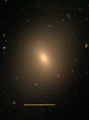
Our view of Elliptical galaxies has changed greatly : [image]
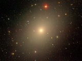 In the 1970s, Ellipticals were thought to be :
- Diskless bulges with deVaucouleurs (R1/4) profiles and constant
density (King) cores.
- Oblate spheroids flattened by rotation
- Void of gas and dust
- Contain a single ancient population of stars
- Relaxed dynamically quiescent systems
To a large extent, all of the above are now thought to be wrong.
(b) Subdividing the Elliptical Class
In what follows, it will be useful to consider three classes of
Ellipticals :
- Luminous : L greater than 1-few L*, MB
brighter than about -20
- Midsize (including massive bulges) : L between 0.1 L* & L*,
MB in the range -18 to -20
- Dwarfs (dE & dSph) : L less than 0.1 L*, or MB
fainter than -18.
Luminous and midsize have somewhat different properties, but form a single
sequence in mass.
Diffuse dwarf Es & dwarf spheroidals are significantly different.
(c) Parameters
Here are a few recurring parameters we need to be familiar with :
- Surface Brightness (SB) : I(R) (flux
units), µ(R) (mag/ss units). IB is for B band, etc
- Total flux : (a) within projected radius L(<R), or (b)
integrated: Ltot (equivalent to MB)
- Effective Radius : Re defined as the half light
radius: L(<Re) = 0.5 Ltot [c.f.
Ie
 I(Re) ]
- Stellar Velocity Dispersion:
 (R)
(R)
Assumes a Gaussian projected stellar velocity distribution
Usually single central aperture [ideally, includes light out to Re, giving
e =
< (<Re
) > ]
Also important, are properties of the core :
- Central Surface Brightness: I0 = I(0)
- Core Radius: rc or Rc, such that I(Rc) = 0.5 I(0)
Sometimes rc (or rb) refers to a break in the near nuclear light profile.
- Central Stellar Velocity Dispersion: o =
(0)
Remember : I(R) is independent of distance ! (for small redshifts).
(d) Deprojection
Note that all the above quantities are projected onto the sky.
Ultimately we want true 3D spatial information. I.e. we want to derive :
- The luminosity density j(r) from the surface
brightness I(R), where
- r is true (3D) radius and R is projected radius
- For constant M/L ratio, j(r) and I(R) track the space and projected
mass densities [i.e.
 (r) and µ(R) ]
In general, with z2 = r2 - R2
and dz = r dr / (r2 - R2)1/2, we have
[image]
 |
(7.1) |
This is an Abel Integral equation, with solution
 |
(7.2) |
- There are a few useful I(R) & j(r) pairs that can both be expressed algebraically
- For smooth (fitted) profiles, evaluate the integral directly
- For noisy data, use the Richardson-Lucy iterative inversion
Note : if the image is elliptical, a unique inversion is only possible
for an axisymmetric figues viewed from the equatorial plane.
Just to orient ourselves, consider a single power law of index
 (typically, 0.5 <
< 1.5)
(typically, 0.5 <
< 1.5)
(e) Observational Concerns
There are a number of practical difficulties facing accurate surface photometry
- Sky Subtraction is critical. Typically one aims for I(R) about
5% to 0.5% of sky.
[image]
Difficult especially with small CCDs which may not extend far enough
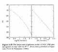
- Seeing affects the central regions: convolving with
the PSF (e.g. Gaussian + PL wings) :
- I(R) turns over into a flat core for R < 1
- Ellipticity decreases significantly for R < 4
- a4 is affected even further out

(2) Radial Light Profiles: Outside The Core
Elliptical galaxy light profiles are relatively similar with important differences: [image]
There is a long history of trying to fit these brightness profiles.
Reynolds (1913) and Hubble (1930) used: I(R) = I(0) / (1 + R/R0)2
A modified form has the benefit of having an analytic deprojected density:
I(R) = I(0) / [1 + (R/r0)2] with j(r) = I(0) / 2r0[1 + (r/r0)2]3/2
Today's preferred fitting functions are a little different.
(a) Fitting Functions
(i) deVaucouleurs (R1/4) and Sersic (R1/n) Laws
deVaucouleurs noticed (1948) that for many ellipticals µ  R1/4
R1/4
The fit is usually good over all but the inner and outermost regions (typically 0.03 - 20 Re)
 [image]
The law is usually written :
 |
(7.3) |
It has the following properties :
- Ltot = 7.22
 Re2 Ie
- I(0) = 2000 Ie
- < I(<Re)> = 3.61 Ie (which we abbreviate
to < Ie > and equivalently <
µe >)
- Asymptotically, at small R, I(R) R-0.8
while at large R, I(R)
R-1.7
- In terms of surface brightness:
µ(R) =
µe +
8.325[ (R/Re)1/4 - 1 ] =
µ(0) + 8.325 (R/Re)1/4
- While originally purely empirical, Binney (1982) has shown that the
R1/4 law arises naturally from a reasonable distribution function.
The deVaucouleurs law is a special case of a more general, Sersic (1963,1968), law:
 |
(7.4) |
Where
It turns out (see below) that different n's fit the different classes of Ellipticals
(ii) Double Power-Law (Dehnen) Laws
An alternative approach is to:
(a) Choose a double power law to match inner and outer slopes
(b) Specify the space luminosity density, j(r), rather than the projected light I(R).
One well-studied example is:
 |
(7.5) |
Clearly, for r << r0 we have j(r) r - and for r >> r0 we have j(r) r - 
Specific models include:
For example the Jaffe model has the following properties:
- ro contains half the unprojected light
- Re = 0.76 ro contains half the projected light
- Expressions for the integrated (aperture) light, and gravitational potential are:
 |
(7.6a) (7.6b) |
- The projected light profile has an analytic form (a=R/ro) :
 |
(7.7) |
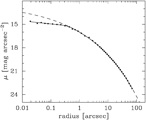
- An example of a Jaffe model fit to NGC 3379 is shown here [image]
(b) Resulting Fits
For many years, the deVaucouleurs R1/4 was the primary fitting function
It now seems there are systematic variation that require the other 3-parameter functions
The nuclear regions are in any case poorly fit, and are discussed separately below.
A recent and very thorough study is that of Kormendy et al (2009 o-link)
(i) Variation with Luminosity
Galaxies of different luminosity have different concentrations (n-index) [image]
The R1/4 law fits best near MB~ -21.
Fitting Sersic profiles to find n-index gives:
- Lower luminosity Es less concentrated, n < 4 (Jaffe ~ 2)
- Higher luminosity Es more concentrated n > 4 (Hernquist ~ 1)
(ii) Variation with Environment
There is some evidence that outer light profiles can be affected by neighbors :
- Ellipticals in dense clusters have profiles that are cutoff
at large radii
likely caused by stars being lost due to tidal evaporation
- Ellipticals with a near neighbor can have a raised outer profile
likely caused by tidal heating which puffs up the outer envelope
(iii) cD galaxies
cD galaxies are well fit by the R1/4 law out to about 20Re
Outside this, their light profiles lie above the fit (eg I(R)
R-1.6),
in an extended halo [image]
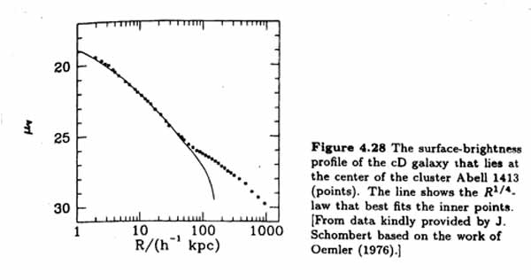
This halo light may not come from the galaxy but from stars in the cluster
- the stellar velocity dispersion increases with radius, as expected
for cluster stars
(note : velocity dispersion usually drops with radius in normal Es)
- the isophotes can change to match the isopleths of the cluster
galaxy distribution.
(iv) Ripples and Shells
About 10% - 20% of Ellipticals have "ripples", of amplitude 3-5%
[image]
These shells indicate recent accretion of disk galaxies (discussed more in Topic 12)
Clearly, mergers play a role in the formation of at least some ellipticals.
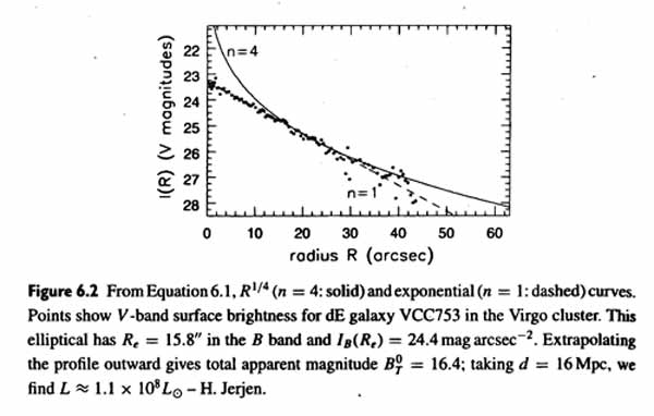
(v) Dwarf Ellipticals & Dwarf Spheroidals
There are two classes of Dwarf Ellipticals :
- Compact dEs : these are quite rare, but are clearly a
continuation of their more luminous counterparts
eg M32 which has a reasonable R1/4 profile, perhaps slightly steeper, as expected.
- Diffuse dEs : these are common and are quite different
from the more luminous Ellipticals
Kormendy calls these "Spheroidals" to keep the distinction clear
They extend in luminosity down to include the Milky Way dwarf spheroidals, like Leo I etc.
These Spheroidals have exponential light profiles (Sersic with
n ~ 1) [image]
(3) Nuclear Regions
It transpires that the nuclear regions are very important:
they give insight into the galaxy's formation history
they can be influenced significantly by a central black hole
Early (pre-1975) work suggested that I(R) turned over in a flat core of constant density
This was naturally understood in terms of isothermal and King models (see below)
However, the serious influence of seeing, especially in photographic work, had not been appreciated.
The existence of flat cores was shown to be incorrect with CCD images (eg Kormendy 1977)
Significant progress was only possible using HST.
In general, the above functions fail to match the nuclear regions very well.
Within a "break radius" there can be deviations both below and above the best fit to the outer parts.
(a) Fitting Functions
(b) Results: Two Types, Cores & Power-laws
For significant samples, "Nuker" profiles were fitted, and showed :
[image]
- There are no cases where I(R) is flat at the center;
all continue to rise down to 0.1 arcsec.
- The inner profiles divide into two groups:
- Power laws: profile keeps rising steeply: j(r)
r-1.9
with I(R) diverging at R=0
- Cuspy cores: profile breaks to shallower power-law: j(r)
r-0.8
with I(R) finite at R=0
- These two types depend on the galaxy's total luminosity:
- Nuclear power laws are found in Lower Luminosity Ellipticals
and Spiral bulges (L < ~L*)
- Nuclear cores are found in Higher Luminosity Ellipticals
(c) Summary: Three Kinds of Ellipticals
There now seems to be three types of "Elliptical" galaxies:
[image]
 In order of increasing total luminosity:
Spheroidals: (diffuse dEs and dSph).
Coreless Ellipticals:
Core Ellipticals:
(4) Scaling Relations
There are many correlations between the various properties of Ellipticals.
The tightness of some are quite remarkable, and point to
an underlying homogeneity of this class of galaxy.
(a) Early 2-Parameter Correlations
(b) The 3-Parameter Fundamental Plane
The above 2-parameter correlations have considerable real scatter
([image], B&M 4.43)
 Furthermore, the residuals in one plot correlate with those in another.
This suggests we look for a tighter correlation among three
parameters:
- A tilted plane of points in 3-D volume, which
- Projects onto 2-D planes as the (looser) correlations seen above
- One example is: Log Re = a Log + b Log Ie + c
The choice of the 3 parameters is not unique
Three choices have been studied --- they are essentially equivalent.
(i) Log Re, <
µe >,
Log e
(Djorgovski & Davis 1987)
Here, Re is in kpc; <
µe > is in
B mag/ss; e
is in km/s
[Note : we could have used
µe rather
than <
µe >
or even Ltot = 2 Le = 2 pi Re2 <
µe > ]
Several statistical methods can identify/characterise correlations in n-dimensions :
- Principal Component Analysis (PCA)
- Multiple Linear Regression
- Partial Correlation Analysis
Using these, we find the equation of the Fundamental Plane to be :
-
Log Re = 0.36 <
µe >
+ 1.4
Log e
+ const
[normal vector (-0.65, 0.22, 0.86) ]
Viewed edge on, the plane has very little scatter ~15% [image]
(ii) The Dn -
Relation
(Dressler et al 1987 : Seven Samurai)
Before the F-P was found, a very tight 2-parameter correlation was identified:
[image]
Dn vs
e, where
Dn = Diameter (in kpc) where <
µ > = 20.75
B mag/ss
 (the actual value of 20.75 is not important)
It turns out that this choice of parameters renders the F-P essentially edge-on
Here's why :
For R1/4 law, integration gives Dn
Re
< Ie >0.8 or, equivalently
-
Log Dn = Log Re + 0.8 Log
< Ie > = Log Re - 0.32 <
µe >
(since <
µe >
= -2.5 Log < Ie > )
Substituting for Re in the F-P relation, we get :
- Log Dn + 0.32 <
µe >
= 0.36 <
µe > +
1.4 Log e
Log Dn = 1.4 Log e - 0.02 <
µe >
and we see that the dependency on
< µe >
has essentially vanished, leaving
Dn
e 1.4
: a tight 2-parameter correlation
(iii) Kappa Space :
 1
2
3
(Bender et al 1993)
1
2
3
(Bender et al 1993)
A deliberate attempt to render the F-P "edge-on" using more physical
parameters:
- 1
=
2-1/2 Log(
e2 Re )
Log M (M = Mass)
- 2
=
6-1/2 Log( e2 Ie2 / Re )
Log [ Ie (M/L)1/3 ]
- 3
=
3-1/2 Log( e2 / Ie / Re )
Log (M/L)
In this K-space we find tight projections in
1 vs
3 [image]
This suggests a narrow range of M/L which correlates weakly with total mass
(iv) The Physical Basis of the Fundamental Plane
The following gives some insight into the origin of the F-P relation :
Consider:
- < Ie > = ½ Ltot / Re2 (just a definition)
- M/Re = c
e2
(virial equilibrium, KE
PE; c = "structure
parameter" containing all details)
Taken together, these give:
- Re = (c/2) (M/L)-1
e2
< Ie >-1 or equivalently,
- Log Re = Log [(c/2) (M/L)-1]
+ 2 Log e - Log < Ie > or
- Log Re = Log [(c/2) (M/L)-1]
+ 2 Log e + 0.4 <
µe >
(since <
µe >
= -2.5 Log < Ie > )
So, if c and M/L are constants, then we expect
- Log Re = 2 Log
e
+ 0.4 <
µe >
+ Log [(c/2) (M/L)-1]
Which is close to, but not quite, the F-P relation:
- Log Re = 1.4 Log
e + 0.36 <
µe >
+ const
To bring these into agreement, we require:
We conclude:
- The F-P is rooted principally in virial equilibrium
- To first order, the M/L ratios and dynamical structures of ellipticals
are very similar
This, in turn, suggests the populations, ages & dark matter properties are
highly uniform
- There is a weak trend for M/L to increase slightly with Mass
(× 3 across 5 magnitudes)
- The actual M/L values, ~10-20 (h=1), are consistent with no
dark matter (within Re)
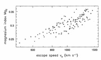
- The narrow scatter on F-P and Mg2 -
relations place
limits on the ranges of ages and metallicities:
Ages ~ 10 - 13 Gyr; Z ~ 2-4 Z(solar)
- None of these relations seems to depend on environment: internal properties are relatively robust
(v) Use of F-P in Distance Measurement
Much motivation for the above work was to improve methods of distance
measurement
In general, if a
 V (km/s) correlates
with a luminosity or size, we have a distance indicator, eg :
V (km/s) correlates
with a luminosity or size, we have a distance indicator, eg :
- Tully-Fisher :
Vrot
vs MI
- Faber-Jackson :
e
vs MB
Both the F-P and the Dn-
relations yield
a physical length (kpc) from SB &
, with low scatter
(~10-15%)
This has been used to derive distances :
- Used in the distance ladder to get Ho
- Used with cz to map the peculiar velocity field and large scale flows
(5) The Shape of Elliptical Galaxies
To first order, isophotes are concentric, aligned, ellipses: [image]
Ellipticity
 = 1 - b/a,
eccentricity e = 1 - (b/a)2 [e =
(2 -
);
= 1 -
(1 - e)½ ]
= 1 - b/a,
eccentricity e = 1 - (b/a)2 [e =
(2 -
);
= 1 -
(1 - e)½ ]
Recall, ellipticals are classified En where n = 10
The apparent ellipticity combines the true shape and
projection effects
Hence, unlike other morphological designations, n (in En) is not intrinsic
(a) 3-D Shapes
We start assuming that surfaces of constant density are ellipsoidal
 |
(7.9) |
where a, b, c may be functions of r
Basic questions :
- Are ellipticals predominently: [image]
- oblate ie a = b > c (flying saucer)
- prolate ie a > b = c (cigar)
- triaxial ie a > b > c (smooth box)
- What is the distribution of true shapes?
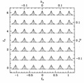
The distribution of observed axial ratios, N(b/a), is shown here: [image]
Note: it has a rise from E0 to E2, followed by a decline to E7
Can we reproduce this from a random orientation of oblate or prolate ellipsoids?
- Projected shape of ellipsoids is more complex than that of disk (eg B&M 4.3.3)
- However, difficult to generate rising distribution from E0 to E2 with just oblate or prolate
- Can be fit by distribution of triaxial, closer to oblate than prolate:
- b/a ~ 0.98 (close to oblate)
- c/a ~ 0.69 (quite flattened)
- each have Gaussian dispersion ~0.11
The conclusion of triaxiality is supported by the presence of isophote twists in many ellipticals:
[image]
- PA of major axis changes with radius (so can
)
- Cannot result from projection of oblate or prolate shapes
- Intrinsically twisted galaxies are not stable
- Can occur if triaxial with axial ratios varying with radius.
(b) Isophote Shapes: Boxy & Disky
- Isophotes are not exact ellipses : typical deviations ~few %
- In general, one can express the isophote as a Fourier series :
 |
(7.10) |
a0 is the mean radius
a1, b1 define the ellipse center
a2, b2 define the eccentricity and position angle
 a3, b3 are useful diagnostics of dust (asymmetries)
Note : a3 and all bn are zero for 4-fold symmetry
a4 defines the boxiness or diskiness (pointiness is better term)
- parameter a4/a0 typically in the range -0.02 to +0.04
[image]
a4 < 0 : boxy
a4 > 0 : disky
The a4 parameters are very important since they correlate with
many other variables (see below, § 8)
(6) Kinematics of Elliptical Galaxies
(a) Methods of Analysis
If stars produced single isolated emission lines, their (projected) velocity
field would be easy to find:
The distribution of projected velocities N(v)
F(
 ) i.e. the
emission line profile
) i.e. the
emission line profile
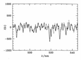
However, Ellipticals have complex absorption line spectra:
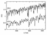 Similar to a K giant, but broadened by Doppler motion of the stars: [image]
Consider :
S() =
Stellar Template = a single star spectrum
N(v) = relative (normalised) number of stars of projected velocity v (ie vlos)
N(v) is usually called the LOSVD (Line Of Sight Velocity
Distribution)
G() = observed (broadened) galaxy spectrum
Loosely speaking, G()
is the same as S()
convolved (smoothed) by N(v)
We observe G()
and S() and try
to obtain N(v).
Details :
- First rebin G()
and S() into u = c Loge
so pixels
u = c Loge = c/ = v, i.e. km/s/pix rather than A/pix
our convolution is, in fact: G(u) = S(u) ® N(u)
(where ® is convolution)
- Sum several template stars to match the overall galaxy stellar
population
 template mismatch is a principle source of error
- Remove low frequencies (e.g. >50A continuum variations) and
high frequencies (noise)
do this in Fourier space: apply filter to FT and transform back
[image]
Several methods have been devised to extract N(v)
(i) Fourier Quotient (Sargent et al 1977)
Writing Fourier transforms (in k space) in bold face :
Starting with the galaxy spectrum :
|
G(u) = S(u) ® N(u) |
(7.11) |
From the convolution theorem we have :
|
G(k) = S(k) × N(k) |
(7.12) |
giving
|
N(k) = G(k) / S(k) |
(7.13) |
We cannot simply inverse transform N(k) because noise is introduced by the division.
Instead, assume N(v) is Gaussian, so N(k) is also Gaussian
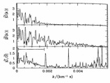 Estimate N(k) by fitting a Gaussian to the quotient [image]
from this fit, we quicky obtain N(v) as a Gaussian
so the LOSVD is characterized by just cz, , and
 (effective line strength)
(ii) Cross Correlation (Tonry and Davis 1979)
It is not difficult to show that:
|
G(u) © S(u) = N(u) ® [S(u) © S(u)] |
(7.14) |
where © is cross-correlation and ® is convolution
(note S(u) © S(u) is also called auto-correlation)
In English: the cross-correlation of the galaxy and template spectra is just
the cross-correlation of the template with itself convolved by the broadening function.
In general, cross-correlating the galaxy and template produces an offset peak
[image]
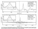
Cross-correlating the template with itself produces a narrower peak at
zero offset
- The offset of the peak from zero gives the redshift
- The difference in shape of the two peaks gives the LOSVD
- In practice, only Gaussians are used to model N(u), yielding
(iii) Other Methods (more recent)
A number of related methods have been devised since these originals
Many try to extract more information from the LOSVD (i.e. deviations from Gaussian)
These characterisations include:
- Sums of Gaussians of different velocity, width, and strength
- Higher classical moments (ie k>2), eg
 k =
µk /
k where
µ is the kth moment
k =
µk /
k where
µ is the kth moment
however, they weight the noisy wings too much, so alternatives are better
- Gauss-Hermite functions: hk (Gaussians multiplied by a poynomial)
Ultimately, we really only deal with two extra parameters for the LOSVD:
[image]
- Skewness (k=3), i.e. asymmetric slope to higher/lower velocities
- Kurtosis (k=4), i.e. stubby/peaky
In practice, these parameters are evaluated as part of an optimized
 2 fit
[image]
2 fit
[image]
to the observed spectrum of the template convolved by a parameterised LOSVD
(b) Amount of Rotation
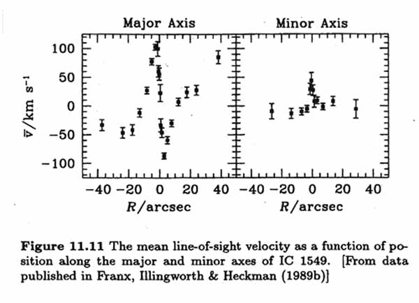
(c) Axis of Rotation
Naively, for an axisymmetric rotating galaxy, one expects:
- Major axis slit should show maximum rotation
- Minor axis slit should show no rotation
- i.e. kinematic axis = photometric minor axis
While for a triaxial rotating galaxy, one expects:
- The projected photometric minor axis need not align with any true axis
- The rotation axis can be anywhere in the plane defined by the longest and shortest axes
What do the data suggest?
Let  = the projected
kinematic misalignment
= the projected
kinematic misalignment
= angle between kinematic
and photometric minor axes
For some fiducial radius, Rf, a good estimate of this is:
 |
(7.17) |
A histogram of est shows:
[image]
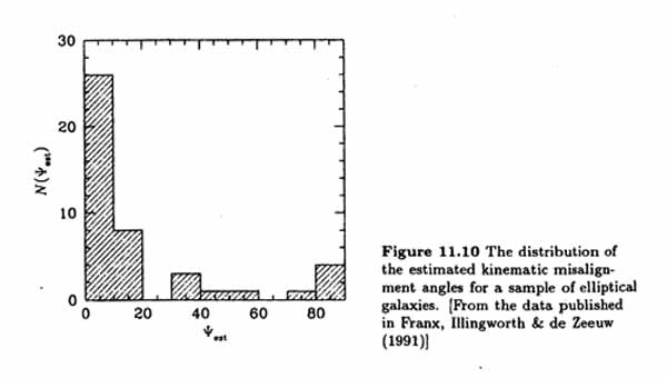
- Most are ~ 0
- Some are 0 - 90
- Significant minor-axis rotation occurs in boxy Ellipticals, suggesting triaxiality.
(d) Kinematically Distinct Cores and Dust Lanes
~25 % Ellipticals show a separate, rotating component
in the nuclear regions (~1kpc; 0.1-0.3 Re)
These are called Kinematically Distinct Cores (KDC)
Projection effects and difficult detection suggest maybe
30%-60% Ellipticals have KDCs.
Here are some examples: [image]
The KDCs show the following :
-
Rapid rotation (Vr / )* > 1,
with a range from "warm" to "cold": Vr / = 1 to 4.5
- Kinematic axis aligned with the photometric axis.
- Some KDCs even counter-rotate relative to the host
Clearly, they have a different (later?) origin than the main galaxy
- They have higher metallicity than the rest of the galaxy [image]
- Photometrically, they are difficult to identify (e.g. not necessarily disky isophotes) :
they don't contain much mass
kinematically prominent in LOSVD because they have low
(e.g. large h3)
-
May be related to subtle gas/dust lanes/disks seen in many (~40%) ellipticals
 Often randomly aligned at large radii but aligned with minor axis at small radii
extreme example (NGC 5128) shown here: [image]
KDCs (and dust lanes) are likely to be a byproduct of dissipational tidal capture
-
Gas and/or star system captured
-
Dissipation (loss of orbital energy) occurs: stellar system decays by dynamical friction;
gas settles, loosing energy by line radiation.
-
Angular momentum (AM) inherited from merger (not from host): at large radii we have random orientation (of gas/dust); at center torques/precession aligns with minor axis.
-
Gas disk undergoes star formation to generates a stellar disk. Stars age and disk becomes photometrically difficult to identify.
Conclusion :
Formation of ellipticals via single event is only part of story
Ongoing mergers/accretion plays at least some role in construction of present-day ellipticals
(7) Mass to Light Ratios
In principle :
Stellar velocities & radius give Mass
Photometry gives Light
Together, we get M/L ratios.
In practice, not so straightforward:
- Ideally, need full velocity distribution function at each location.
- Now possible to build reasonable models using LOSVD (see Topic 8).
- Usually, however, we need to assume nearly isotropic velocity field.
(a) Inner Parts
Simple estimates:
Assume approximately isothermal and fit a King profile (sec 3a above)
We find a central luminosity density, central mass density, and central M/L:
- j(0) = I(0) / 2ro
- (0) =
9 (0)2
/ 4 G ro2
- M/L = 9 (0)2
/ 2 G I(0) ro
Typically, M/L ~ 10 h M / LB,
so dark matter does not dominate in the center.
/ LB,
so dark matter does not dominate in the center.
(b) Outer Parts & Halo
(8) Two Kinds of Ellipticals : Boxy and Disky
Summary of properties which differ for boxy
(a4 < 0) and disky (a4 > 0) ellipticals
and bulges :
| Property | Boxy (a4 < 0) | Disky
(a4 > 0) |
| Luminosity | high : MB < -22 | low :
MB > -18 |
| Rotation Rate |
slow/zero :
(Vr / )* < 1 |
faster :
(Vr / )* ~ 1 |
| Flattening | velocity anisotropy | rotational |
| Rotation Axis | anywhere | photometric minor axis |
| Velocity Field | anisotropic | nearly isotropic |
| Shape | moderately triaxial | almost oblate |
| Core Profile | cuspy core | steep power law |
| Core Density | low | high |
| Radio Luminosity | radio loud and quiet
1020 - 1025 W/Hz | radio quiet
< 1021 W/Hz |
| X-ray Luminosity | high | low |
Some of these are shown here: [image]
Note that to first order : Boxy and Disky galaxies have the same :
- color-magnitude relation
- Mg2 vs
relation
- Fundamental Plane relation
It is still unclear quite how to interpret this dichotomy :
The two types may be closely related, or may have quite different histories
Semi-empirically, Kormendy and Bender suggest a modified
Hubble diagram
[image]
- Disky Ellipticals form an extension of the S0s
- Boxy Ellipticals lie at the extreme left end
they may or may not be related to the other ellipticals and S0s
This all has important implications for Elliptical Formation
(9) Formation of Ellipticals
(Note Mergers and Galaxy Formation discussed more in Topics 12 & 19)
Still unclear -- but we have made progress
(a) Two scenarios discussed
(i) Monolithic Dissipative Collapse
- Early massive gas cloud undergoes dissipative collapse
- Huge starburst during collapse
Note: sub-mm detections of ~1010 M
cold gas at
z ~ 2-3 with high SFR.
- Clumpiness during collapse
 violent relaxation ~ isothermal
incomplete violent relaxation non-isothermal & non-isotripic
- Probably rotate "rapidly" "Disky" Ellipticals ???
(ii) Hierarchical Mergers
- Early universe much denser: e.g. z ~ 2 density ~ 27 times higher than today.
Mergers/interactions probably common.
- Sequence of galactic mergers, starting with pre-galactic substructures
- Galaxies continuue to grow during z ~ 1-2
Note : HST finds old ellipticals at z ~ 0.5
- Galaxies fall into clusters and merging ceases (encounter velocities too high)
- Random accretions low AM & anisotropic "Boxy" Ellipticals ???
(b) Relevant Issues & Problems
(i) The Need for Dissipation (loss of energy)
- High stellar densities require dissipation during formation
- eg collapse factors of ~10 needed to convert spiral disks to elliptical cores
- eg at MB ~ -16, Dwarf Spiral vs M32 we have rc ~ 700pc vs
1pc and µ(0) ~ 23 vs 11
- Unlikely/impossible by mergers of stellar systems alone
such mergers cannot increase the (phase-space) density
- Dissiptation requires gaseous collapse/merger & subsequent star formation
(ii) Observational Support for Importance of Mergers
- Ongoing mergers are seen (eg NGC 7252, NGC 6240, Arp 220)
- They have ~ R¼ profiles (in K light)
- Have high central (gas) densities ~102
Mpc-3
comparable to Ellipticals of similar total mass
- Lie close to the F-P for Ellipticals ( from CO; photometry in K)
- Brightest cluster galaxies are clearly accreting (eg multiple nuclei)
- Ongoing accretion is common in ellipticals:
- KDCs
- gas/dust lanes in non-equilibrium configurations
- ripples & shells
(however, don't confuse minor accretion with major merger formation).
(iii) Theoretical Support for Importance of Mergers
- Compact groups have expected lifetimes ~108-9yr
must merge
- N-body simulations of major mergers of two bulge/disk/halo galaxies
R¼
however, highest densities inherited from pre-existing bulges
- N-body simulations of mergers including gas (in SPH
formalism) and star formation (SFR (gas)1.5)
yields:
rapid gas collapse to center (before merger complete) with nuclear starburst
final profile: dense core with "break" in power-law
(iv) Problems to Overcome
- Dense nuclei survive mergers - so why do giant Es have
larger lower density cores if built from denser bulges and Es?
- Mergers of Es &/or bulges should destroy the F-P
- GC frequency (per unit luminosity) is ~25 times higher in Es than Spirals
(maybe GCs form during merger - e.g. as in NGC 1275)
- difficult to generate metallicity vs luminosity correlation by merging
lower luminosity systems
(unless metals made during merging starburst)
(c) Hybrid : Merger Induced Dissipational Collapse
 Kormendy & Sanders (1992) combine the two formation scenarios:
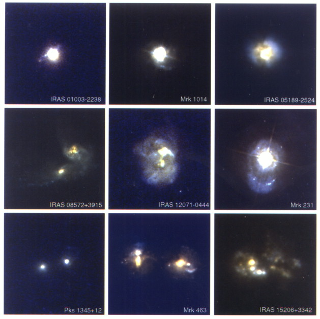
Similar to Ultra-Luminous Infra-red Galaxies (ULIRGs; e.g. Arp 220 etc;
[image] )
- They are mergers, showing tidal debris etc
- They have high central densities ~102 Mpc-3,
similar to the central stellar densities of ellipticals
- They have similar gas mass and stellar mass in the central regions
dissipation has occurred, sending the gas to the center
- There is a huge ongoing starburst, creating a homogeneous metal rich population
We have, in these systems, a substantial dissipative collapse which is associated with a major merger
They speculate that the ULIRGs are ellipticals caught in formation
Interestingly, ULIRGs are also thought to be proto-quasars :
- feeding (and possible creation of) nuclear black holes
- star formation luminosity comparable to quasar luminosity
- currently hidden by dust (which re-radiates in the far IR)
- ultimately becomes visible when surrounding gas swept clear
The ULIRGs are locally rare - maybe they were common at high-z
Elliptical formation may be associated directly with the quasar era ?
 -2 (R/Re)1/n
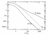

 =
tangential velocity dispersion (assume
=
tangential velocity dispersion (assume
 =
=
 ) : M(r) = 2