Whittle : EXTRAGALACTIC ASTRONOMY

 
     
 

1 : Preliminaries	6 :   Dynamics I	11 : Star Formation	16 : Cosmology
2 : Morphology	7 :   Ellipticals	12 : Interactions	17 : Structure Growth
3 : Surveys	8 :   Dynamics II	13 : Groups & Clusters	18 : Galaxy Formation
4 : Lum. Functions	9 :   Gas & Dust	14 : Nuclei & BHs	19 : Reionization & IGM
5 : Spirals	10 : Populations	15 : AGNs & Quasars	20 : Dark Matter

(1) Introduction

• First, some similarities :
  Each comprise many, interacting objects which act as points (separation >> size)
  Each can be described by distributions in space and velocity
  eg Maxwellian velocity distributions; uniform density; spherically concentrated etc.
  Stars or atoms are neither created nor destroyed -- they both obey continuity equations
  All interactions as well as the system as a whole obeys conservation laws (eg energy, momentum)

• Now some crucial differences :
  The relative importance of short and long range forces is radically different :
  -- atoms interact only with their neighbors, during brief elastic repulsive collisions
  -- stars interact continuously with the entire ensemble via the long range attractive force of gravity
  e.g. uniform medium: F     G dr / r²     r²dr / r²     dr    equal force from all distances
  The relative frequency of strong encounters is radiaclly different :  
  -- for atoms, encounters are frequent and all are strong (ie V ~ V)
  -- for stars, pairwise encounters are very rare, and the stars move in the smooth global potential.

• Consequently, there are many parallels between gas (fluid) dynamics and stellar dynamics :
  ---> concepts such as Temperature and Pressure can be applied to stellar systems
  ---> we use analogs to the equations of fluid dynamics and hydrostatics

• there are also some interesting differences
  ---> pressures in stellar systems can be anisotropic
  ---> stellar systems have negative specific heat and evolve away from uniform temperature.

• The geometry of gravitational potentials is a good starting point :
    methods to derive gravitational potentials from mass distributions, and visa versa.

• Potentials define how stars move
    consider stellar orbit shapes, and divide them into orbit classes.

• The gravitational field and stellar motion are deeply interconnected :
    the Virial Theorem relates the global potential energy and kinetic energy of the system.
  The Virial Theorem can be used to investigate :
    the masses of stellar systems
    how energy is released during gravitational collapse
    how self-gravitating systems have negative specific heat.
    how the ratio of rotation to dispersion support can define galaxy flattening.

• A more detailed approach requires us to work with a Distribution Function   (DF) :
    the DF specifies how stars are distributed throughout the system and with what velocities.

• For collisionless systems, the DF is constrained by a continuity equation : the CBE
  This can be recast in more observational terms as the Jeans Equation.
  The Jeans Theorem helps us choose DFs which are solutions to the continuity equations.

• With these DFs, we can construct self-consistent models of equilibrium stellar systems.
  Some simple systems are considered in detail, while more complex ones are touched on.

• We introduce situations where the potential is changing in time
  Usually this is untreatable, except when the changes are rapid and large : violent relaxation
  This is important in describing galaxy formation and galaxy merging

• Finally, we relax the collisionless assumption and introduce star-star interactions
    such systems are described by the Fokker-Planck equation
  This reveals a number of slow processes which occur in dense stellar systems :
    2-Body relaxation & equipartition
    Core collapse & the gravothermal catastrophe
    Evaportion & ejection

• Additional important themes are postponed to later Topics :
    Effect of nuclear black holes on stellar distributions (9)
    Dynamical friction (15)
    Tidal evaporation (15)
    Slow (adiabatic) and Fast (impulsive) encounters (15)
    Merging & satellite accretion (15)

(2) Potential Theory

• We initially characterize mass distributions as smooth functions (r)
  (this is usually legitimate for galaxies, see § 8.10 below)

• The gravitational potential energy is a scalar field
  its gradient gives the net gravitational force (per unit mass) which is a vector field :

  (8.1a)         (8.1b)

• evaluating the divergence of F(r) gives :

  (8.2a)       (8.2b)       (8.2c)

  8.2b is Poisson's equation, for locations within the mass distribution
  8.2c is Laplace's equation, for locations outside the mass distribution

• For a volume V with surface A enclosing mass M we have (using Divergence/Gauss's Theorem) :

  (8.3a)         (8.3b)

• Since the force field is the gradient of a potential, it is conservative,
  ie the energy required to move mass from r₁ to r₂ is independent of the path
  the total Potential Energy is therefore well defined
  setting = 0 at r = we get (B&T-2 p 59) :

  (8.4)

  Note that, with this definition, potential energy is always negative

(i) Point Mass

(r) = - GM / r   ;   F(r) = - = -d/dr = -GM / r²
V_c²(r) = GM / r = - (r)   ;   V_esc²(r) = 2GM / r = - 2(r)
where V_c & V_esc are the circular and escape velocities, respectively. 
This is called a Keplerian Potential, since it pertains to the solar system.

(ii) Uniform Spherical Shell

Outside : (r) = - GM / r   (Keplerian)
Inside : (r) = const   ;   F(r) = 0


(iii) Homogeneous Sphere

Sphere radius = a, with (r) = const (r < a)
Outside : (r) = - GM / r   (Keplerian)
Inside : (r) = -2G(a² - r²/3)   ;   F_r = -G M(r) / r² = -(4/3) G × r
which gives SHM with period P_r = (3 / G)^½     and free-fall t_ff ~ ¼ P_r ~ (G)^-½
V_c = [(4/3)G]^½ × r   so that   (r) = const       solid body rotation
note also that P_c = P_r

(iv) Logarithmic Potentials from Flat Rotation Curves

Many rotation curves are flat at large radii : V_c = V_o, so we have :

(8.5)

(v) Spherical Systems

• Power Laws : = _o (r/a)^-
  have M(<r) = (4 G a³ _o) / (3 - ) × (r / a)^3-
  and (r) = -(4 G a² _o) / [(3 - )( - 2)] × (r / a)^2- = V_c² / ( - 2)
  = 3 is a break point:
  For   >   3,   M(<r)   for r 0 : we have infinite mass at the origin.
  For   <   3,   M(<r)   for r : mass diverges at large r.
  However for 2 < < 3 the potential is finite, as are V_c and V_esc, at all radii.
  The case   =   2 is special : it is the singular isothermal sphere
  with V_c   =   (4 G a² _o)^½   =   const at all radii, yielding (r) = 4 G a² _o ln(r / a)
  See § 8.8a,b,c for other isothermal and related (King) spheres [link]

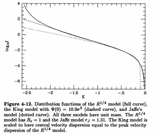
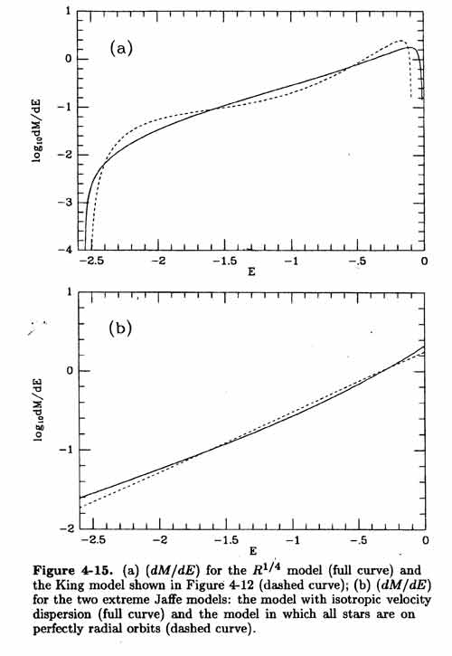
• Hernquist (1990) and Jaffe (1983) models: have r^-4 at large r
  which fits E gals well, and is theoretically grounded in violent relaxation
  at small r, Jaffe core is steeper than Hernquist core :

  (8.6a)         (8.6b)

• Plummer (1911) Sphere: is analytic solution of hydrostatic support for
  polytropic stellar system of index 5; see § 8.8a : [link]
  (r) matches GCs well, but is too steep at large r for Ellipticals ( r^-5).

  (8.7)

• Plummer; Isothermal; Jaffe; and Hernquist density laws are shown here: [ image]

  (vi) Axisymmetric Thin Disks

• Before considering global potentials for disks, first consider the vertical potential near z = 0
  We have two conditions :
  
  within a disk of volume density _o near the plane
  above a disk of surface density
  Using equation 8.3b we have :

  (8.8a)       (8.8b)

• Usually, calculating global and F for disks is algebraically dense.
  Unlike spherical systems, disk potentials usually depend on mass outside R.

  Here are two examples :

• Mestel's disk : (R) = _o R_o / R, has constant V_c : V_c²(R) = 2G_o R_o = GM(<R) / R
  this is unusual in that V_c(R) doesn't depend on mass outside R

• Exponential disk : (R) = _oexp(-R/R_d)
  this fits the light profile of sprial disks much better than Mestel's disk, and has circular velocity

  (8.9)

  where y = R / 2R_d, and I_n K_n are Bessel functions or the 1st and 2nd kind
  see [Topic 5.6a] for an analytic approximation and rotation curve.

  (vii) Axisymmetric Flattened Systems

  Spirals with bulge and disk are, of course, neither just spherical nor just thin disks
  We need potentials which are both combined, ie flattened potentials

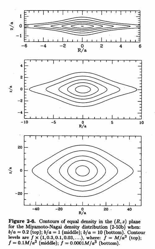
• Miyamoto-Nagai (1975) flattened system [ images ]:
  reduces to the Plummer model if a=0 and the Kuzmin disk if b=0
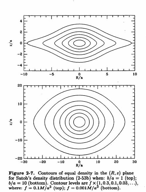
  (Satoh flattened systems are derived in similar manner to the Toomre disks) [ images ] :

  (8.11a)         (8.11b)         (8.11c)

  (viii) Triaxial Ellipsoids

• more complicated, (see B&T-2 § 2.5)

  (ix) Multipole Expansion

  An arbitrary mass distribution sums of spherical shells of non-uniform surface density.
  Calculating the potential involves solving ² = 0 in spherical polar coordinates
  Solutions involve spherical harmonics : Y_l,m (, ) P_l^|m|( cos ) exp(i m )
  where P_l^|m|(x) are associated Legendre functions.
  The potential (r,,) is the sum of a monopole (l=0), a dipole (l=2) quadrupole (l=4) etc...
  each with associated amplitudes

(3) Orbit Classes

(4) Numerical N-Body Methods

• Often, astrophysically interesting systems are algebraically intractable
  Computational methods provide a way forward

• Ironically, employing the Newtonian force law can be a disaster
  "hard" force law (r)^-2
  close encounters give big accelarations and require small timesteps to follow
  if a tight binary forms, this can be a computational sink

• so "soften" the force law (r / (r ² + ²)^-3/2
  (note : this may be inappropriate for small systems where "collisions" are important)

• Direct Summation of pairwise forces
  only posible for N < 50000 ;   ~ O(N²) operations per timestep

• Divide region into cartesian cells : population in each cell changes
  (r)^-2 only evaluated once
  summing done using FFTs since _i = M_j G (r_ij)^-2 (j=1,N) resembles a convolution
  takes (2N)²[1 + 4log₂(2N) ]² steps compared to N⁴ so very efficient for N > 16.
  Typically, 32 × 32 × 32 cube (32768 cells) with 10⁵ stars
  doesn't work well for strong density gradients (eg E's) or galaxy collisions (many empty cells)
  for centrally concentrated disks, choose polar grid spaced in Ln(R) and

• Express potential of mass at r,, by series of spherical harmonics (l < 4 often sufficient)
  calculate total potential by summing these over all particles
  resolution naturally better near nucleus
  ~ N calculations per timestep so very efficient.

(5) The Virial Theorem

We begin by looking at two illustrative cases and then deal with the general case.

(a) Simple Illustrations

(i) Circular Orbit

• Consider a satellite mass m in circular orbit about M (>>m)   : m V² / r = G m M / r²
  multiply by r :   m V² = G m M / r         2K = -W   or   2K + W = 0
    = K / |W| = ½ and E = - K
    Kinetic energy is half the (-ve) potential energy
    The total energy E = K + W is -ve and equal to (minus) the kinetic energy

• As we shall see, = ½ is a characteristic shared by a wide range of systems.
  Note that in this case, the instantaneous values are also equal to the time averaged values
  

  (ii) Time Averaged Keplerian Orbit

• In general, = K / |W| changes along a Keplerian orbit path [image].
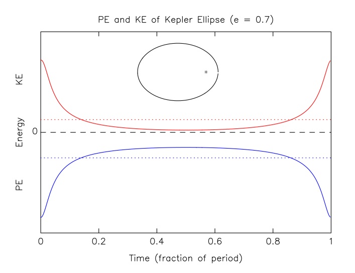
  e.g. compare at pericenter and apocenter :
  
  _p / _a = r_a / r_p 1   (using r_p V_p = r_a V_a from AM conservation) 

• However, taking time averages over an orbit, we find :
  < -W > = < GM/r > = GM < 1/r > = GM × (1/a),   and
  < K > = < ½ V² > = GM < (1/r - 1/2a) > = ½GM × (1/a)
    and we recover, once again : < > = ½ and E = -< K > 

• Note that time averages for single non-Keplerian orbits do not usually have <> = ½
  As we will see, however, = ½ always holds when we average over all particles in a system
  For our Keplerian orbit, m and M are the whole system (with M having ~zero KE)

• There are 3 equations of motion for member (i represents x, y, z) :

  (8.12)

• take the 1st moment in position : multiply by r_j and sum over (j represents x,y,z)
  dimensionally, we have changed an equation of forces into an equation of energies
  after some algebra, we get a set of 9 equations
  these can be neatly written using 3 × 3 matrices (i.e. tensors of order 2)
  this set of equations constitute the Tensor Virial Theorem :

  (8.13)

  where the five tensors are :

  (8.14)   (a,b,c,d,e)

  where _i,j arises from the expansion: <v_i v_j> = <v_i><v_j> + _i,j²

• For steady state systems, d²I_ij / d t² = 0   and we get

  (8.15a)

  the Kinetic and potential energies are related for each tensor element  
  for example, they are related separately along each axis 
  

• Considering just the diagonal terms, we also have :
  Trace(T)   +   ½ Trace()     K   =   total kinetic energy, and
  Trace(W)     W   =   total potential energy
  so for the static case, we get the Scalar Virial Theorem :

  (8.15b)

• Considering the total energy, E, we find :

  (8.15c)

  So the total energy is negative : the system is bound !
  its value is equal to either
  

  minus the (+ve) Kinetic Energy, or
  half the (-ve) Potential Energy

• Here is a very useful little diagram to illustrate the situation : [image]

• Briefly reviewing the conditions necessary to use these simple equations :
  the system must be self gravitating
  the system must be in steady state (orbit timescale << evolution timescale)
  quantities must be time averaged (or many objects sampled with random orbital phase)
  the system must be isolated (or at least embedded in a slowly varying potential)
  Note that the system may be either collisionless (stellar) or collisional (gaseous)

• The most famous use of the virial theorem is to determine the masses of stellar systems.
  For a system of total mass M and mean squared velocity <v²>, K is simply ½ M <v²>
  The virial theorem then gives :
  <v²>   =   -W / M     GM / R_g
  which in practice defines the gravitational radius: R_g

  Knowing R_g and measuring <v²> allows us to determine M, the system mass.
  What to use for R_g isn't obvious for most stellar systems with no clear "edge" or "size"  
  However, we can make use of the median radius : R_m which encloses half the mass
  For many stellar systems, it turns out that R_g     R_m / 0.4   (note R_m is written r_h in B&T)
  We then have :

  (8.16)

  which resembles the circular orbit relation: M = V² R / G, but applies to a general self-gravitating system.

• If the system starts very spread out and at rest :   E   =   K   =   W   =   0
  After settling down, we have once again :   E   =   K   +   W   =   - K
    energy must be released if the system collapses
    this is termed the binding energy, and is the amount needed to unbind the system
    the value of the binding energy is equal to the remaining KE
    the total gravitational energy released is -W, of which
        half goes into KE, and half escapes the system
  Here is another little diagram to illustrate the situation : [image]

• Examples :
  • Collapsing protostars are luminous   they radiate half their gravitational potential energy
    
  • Kelvin considered a gravitational origin for the Sun's energy, via gradual contraction
    
  • For a galaxy, K   ~   ½ M_g V_c²   ~   10⁵⁰ J     10¹⁰ L × 10⁷ years,
    this is 3×10^-7 of the rest mass,   ie (V_c² / c²) × Mc²
    this is negligible in galaxy/starburst formation (nuclear burning is ~7×10^-3 Mc²)

Because gravitational energy is negative, bound systems have negative specific heat:
• Try to slow Earth's orbital motion by pulling back (i.e. remove orbital energy),
        it falls in to lower orbit and speeds up!
• Collapsing gas cloud radiates energy, collapses further, and heats up.
• Add energy to a star cluster (e.g. by accelerating the stars):
        the cluster expands and cools.

Here are diagrams to illustrate the situation : [image]

• Consider an axisymmetric system rotating about the z axis
  By symmetry :
  
  T, , and W are all diagonal
  x & y elements of these tensors are the same

• The tensor virial theorem gives :
  
  2 T_xx   +   _xx   +   W_xx   =   0
  2 T_zz   +   _zz   +   W_zz   =   0
  

• We also have :
  
  T_zz   =   0   (rotation about z     no drift     to z)
  2 T_xx   =   ½ <V>² d³r   =   ½ M V_o²   (V_o is the mass weighted rotation speed)
  _xx   =   M _o²   ( _o is the mass weighted dispersion)
  _zz     (1 - ) _xx   =   (1 - ) M _o²   (   <   1, measures anisotropy)
  W_xx / W_zz     (A/B)^0.9   =   (1 - ) ^-0.9   (A/B is axis ratio of isodensity surfaces)

• Finally, substituting all these into the ratio of the two tensor relations above, we get :
  

  (8.17a)

  B&T-1 fig 4.5 shows this relation for several , including projection corrections [image]
  For isotropic velocities,   =   0, and we get, for small :

  (8.17b)

• In this case, the inclination corrections to V_o / _o and are similar, so the prediction is robust
  

• Observationally, in Topic 7 we found (B&T-1 fig 4.6; [images]
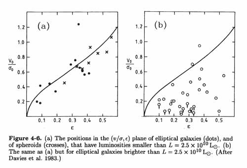
    Low luminosity Ellipticals and Bulges follow the isotropic relation
    Luminous Ellipticals often fall in the anisotropic ( > 0) region

(6) Describing Collisionless Systems

• "Collision", here, means star-star deflection, not direct impact
  For the collisionless case, stars are assumed to move in a completely smooth potential
  (in § 8.10 we consider when and how star-star encounters are relevant).
  Let's briefly justify why this is the case.

• Consider the chances of actual star-star collisions in the solar neighborhood:
  A typical star size/separation is: size ~D(sun) ~1/100 AU (sun ½ deg);   sep ~1pc ~10⁵AU
    Size/sep ~10^-7 filling factor ~10^-21   (note, for air : 10^-1.5 & 10^-4.5)
  Illustration:   star = fine grain of sand (~0.1mm) typical galaxy ~10¹¹ = cubic yard of sand
  But, each separated by ~1km (10m in nucleus)     fills Earth     very empty.
  [Note: since dynamical time t ~ 1 / (G )^½   & _sand ~ _star, then
  the sparse sand model & MW galaxy have the same gravitational timescale:   ~100 Myr ].

• Path length: 1/n = sep³/size² = (sep/size)² x sep = 10¹⁴pc ~10⁹ orbits!
  Collision time: ~10¹⁷yrs @ 200 km/s (~10¹⁸yrs @ disk dispersion).
  Hence the famous statement: when two galaxies collide, no stars collide.
  Alternate perspective: typical star-star encounter deflection ~½ arcsec
  Hence, star orbits follow smooth potential. [movie].

• Notice that Dark Matter (elementary particles) also behaves in a collisionless manner.
  Strange: usually view particles as bouncing around, but these move on smooth orbits
    to first order, DM particles and stars share similar dynamics.
  However, DM currently more extended, so how did this arise?
    gas behaves differently   settles before forming stars.

• A system is fully described by its distribution function (DF) or phase space density :
  f(r, v, t)d³rd³v   =   number of stars at r with v at time t in range d³r and d³v

• Knowledge of the DF is a holy grail, since it yields complete information about the system
  In practice, however, we only observe certain projections of the DF (eg (R), V_p(R), _p(R) )

• Recovering the DF directly from observations is essentially impossible.
  To proceed, we need to introduce further constraints on the DF :
  an obvious example is f(r, v, t) > 0 everywhere and always, ie we cannot have -ve # stars !

  However, there are other constraints :

• Look for a continuity equation, since :
  no stars created/destroyed : flow conserves stars
  stars do not jump across the phase space (ie no deflective encounters)
  View the DF as a moving fluid of stars in 6-D space (r, v),   ie x,y,z,v_x,v_y,v_z
  stars move/flow through the region as their positions and velocities change
  

• Consider a 1-D example using x and v_x, and recall f is a number density
  focus on a small element of phase space at x and v_x with size dx by dv_x
  this [image] will help visualize the situation

• In interval dt, net flow in x is :

  (8.18a)

  the net flow due to the velocity gradient is

  (8.18b)

  the sum of these equals the net change to f in the region, ie at x, v_x of size dx dv_x

  (8.18c)

  or, dividing by dx dv_x dt, we get

  (8.19a)

  but since

  (8.19b)

  we have

  (8.19c)

  adding the y and z dimensions, which are independent, we finally have

  (8.19d)

  This is the collisionless Boltzmann equation (CBE)

• The CBE describes how the DF changes in time
  It is a direct consequence of :

  1  conservation of stars  2  stars follow smooth orbits  3  flow of stars through r defines implicily the location v   (= dr/dt)    4  flow of stars through v is given explicitly by -

• Since f/t is a Eulerian (partial) differential, it describes the change in DF at a point in phase space

• However, consider the Lagrangian (total, or convective) derivative : Df/Dt df/dt.
  This describes the change in f as we follow along the "orbit" through phase space
  But, this Lagrangian derivative is nothing more than the LHS of the CBE

  (8.20)

  Clearly, the phase space density (f) along the star's orbit is constant
  ie the flow is "incompressible" in phase-space
  for example
  

  if a region gets more dense, will increase
  if a region expands, will decrease
  example -- marathon race : start : n high, v high ; end : n low, v low

• The CBE applies to all sub-populations of stars (eg each spectral class)
  even though no single class determines the potential
  in § 8.7b we introduce a self-consistent f which itself generates :

• As it stands, the CBE is of rather limited use :
  
  • the constraints it provides are still insufficient to find f(r,v,t)
    
  • the complexity of f(r,v,t) renders it observationally inaccessible.

• What we observe are :
  • mean velocities   :   < v >
  • velocity dispersions   :     (which is related to < v² > ) 
  • stellar densities   :   n   (also for mass density, or j for luminosity denisty)
  We need to recast the CBE in terms of these quantities. 

• Clearly, these observable quantities are contained within the DF : f (r,v,t)
  they can be extracted by taking appropriate averages or moments
  for example :
  number density   =   n(r, t)     =   f(r, v, t) d³v               =   0th moment in v
  mean velocity   =   <v_i(r, t)>   =  (1/n) v_i f(r, v, t) d³v   =   1st moment in v
  

  If we take moments of the CBE, we transform it into equations in these new variables.
  Lets look in more detail at these first two moments in v (see B&T-2 §4.8) :

• Using the 1-D x axis as example, simply integrate the CBE (eq 8.19c) over all v_x
  We obtain (0th moment in v_x) :

  (8.21)

  where n n(x,t) is the space density and <v_x> is the mean drift velocity along x
  This is a simple continuity equation for the number of stars along the x axis.

• Now multiply the CBE (eq 8.19c again) through by v_x and again integrate over all v_x
  on rearranging and using eq 8.21 above, we obtain (1st moment in v_x) :

  (8.22a)

  where _x² is the velocity dispersion about the mean velocity,
  it arises from <v_x²>   =   <v_x>² + _x²

• repeating this in 3-D requires a little care (B&T-2 § 4.8) :
  we obtain the Jeans Equation (for coordinate j) :

  (8.22b)

  where the summation convention applies (sum over repeated indices)
  here, i=1,2,3 and j=1,2,3 refer to x,y,z,  eg x₂ y and v₂ v_y

• This Jeans equation is akin to Newtons's second law : dv/dt = F/m   with :
  LHS is the derivative of <v>
  RHS are force terms

• It is instructive to compare this to Euler's Equation for fluid flow :

  (8.23)

  which is clearly analogous.

• In 8.22b  n _i,j² is a stress tensor which takes the role of an anisotropic pressure
  (hence the phrase "pressure supported")
  in a fluid, pressure is a scalar and is therefore always isotropic
  for stellar systems, _i,j is a tensor which can be anisotropic

• _i,j is symmetric, : i.e. axes exist where _1,1, _2,2, _3,3 are semi-axes of a velocity ellipsoid
  if _1,1 = _2,2 = _3,3 we have isotropic dispersion     Jeans and Euler equations are identical

• For collisionless systems there is no equation of state linking pressure (_i,j²) to density
  Usually, therefore, we are forced to assume _i,j (or, equivalently, the anisotropy parameter )
  Recently, however, the LOSVD has been used to constrain   (see T 5.7a : [link]).

-- deriving M/L profiles in spherical galaxies (B&T-1 4.2.1d)
-- deriving the flattening of a rotating spheroid with isotropic velocity dispersion (B&T-1 4.2.1e)
-- analysis of asymmetric drift (B&T-1 4.2.1a)
-- surface density (and volume density) in the galactic disk (B&T-1 4.2.1b)
-- analysis of the local velocity ellipsoid in terms of Oort's constants (B&T-1 4.2.1c)

Here we look briefly at the first and second :

(i) Spherically Symmetric Steady State Systems

• This is, of course, an important special case to consider :
  For steady state, the first term in Eq 8.22b is zero
  For spherical symmetry : <v_r> = <v> = 0,   giving < v_r² > = _r²   and   < v² > = ².
  After transforming to spherical polar coordinates, the Jeans Equation reads    :

  (8.24a)

  Introducing anisotropy parameters   :   = 1 - ² / _r²   and = 1 - ² / _r²
  and writing 2 for +   and V_rot for <v >   this becomes

  (8.24b)

  which is equivalent to the equation of hydrostatic support : 
  dp /dr   +   anisotropic correction   +   centrifugal correction   =   F_grav
  

• Going a little further, recasting d / dr   as   GM(<r) / r² = V_c² / r   (V_c = circular velocity)
  and rewriting the first term in eq 8.24b in logarithmic gradients, we have : 

  (8.24c)

  This parallels the equation for hydrostatic support of an ideal gas, where p = nkT
  the equivalences are :

  _r²     T
  d(ln n) / d(ln r)  +   d(ln T) / d(ln r)     (n/p) dp / dr
  2   and V_rot²   are anisotropy and rotation correction terms

• By measuring brightness profiles and velocity dispersion & rotation profiles,
  we can derive (assuming ) : M(r) and hence M/L (r)
  This is very important, eg, in the search for nuclear black holes (see Topic 14.2 : link)

  (ii) Rotational Flattening Revisited.

  TBD

  (iii) Vertical Disk Structure.

  TBD

(7) Steady State : The DF as   f(E, |L|, L_z)

The answer is yes, by introducing two new powerful constraints :
  demand that the system is in steady state   ( in equilibrium)
  demand that the DF generate the full potential   (not just act as a tracer population)

We consider these in turn

(a) Integrals of Motion and the Jeans Theorem

• When a system is in steady state, and f are not explicit functions of time
  In this case, we may introduce a powerful new entity : Integrals of motion
  An "integral of motion" is a function I (r, v) which is constant along a star's orbit (B&T-1 § 3.1.1)
  Obvious examples of possible integrals of motion are :

  E (r, v) =   ½v2 + (r) =   energy per unit mass   in a static potential     L (r, v) =   r × v =   total AM in a spherical static potential     Lz (r, v)   =   (x2 + y2)½ v =   z component of AM in an axisymmetric static potential

• Since I (r, v) is constant along an orbit, it is also a solution to the steady state CBE
  specifically :

  (8.25)

• Since the CBE is a linear equation, then functions of solutions are themselves solutions
  This yields the Jeans Theorem :

  Any function of integrals of motion f (I1, I2, I3, ..... ) is also a solution of the steady state CBE

• This is extremely useful since it allows us to construct legitimate DFs using integrals of motion :
  eg,: the DF : f (E, L_z) = N_o (E² + 3L_z^5/2) is a solution to the CBE for an axisymmetric potential

• In the special case of steady state spherical systems, it is easy to show (B&T-1 § 4.4.2) that :
  • DFs must have the form f(E, |L|)
  • DFs of the form f(E) must have an isotropic velocity dispersion _r  =     =  
  • DFs of the form f(E, |L|) must have an anisotropic velocity dispersion _r       =  

• Summarizing: these theorems provide a very useful way to begin constructing working models :
  For each r and v location in phase space calculate, for example, E, |L|, L_z
  Now assign the number of stars at that location in phase space, f(r,v), by some function of E, |L|, L_z.
  These DFs now automatically satisfy the continuity condition expressed by the steady state CBE.

• Both the CBE and the Jeans Equation include a potential gradient,
  In neither equation, however, are these potentials linked explicitly to the DF
  (recall f(r, v) d³v   =   n(r)     (r) which could, in principle, define )
  As it stands, the DFs only describe tracer populations. 

• Clearly, an important step is to require that the DF also yields the potential (r)
  ie :

  (8.26a)         (8.26b)

  where f here is the mass DF (ie we've multiplied f by the mean stellar mass)

• Taking the spherical form for ², this reads   (eg for a DF of the form f (E, |L|)   :

  (8.27)

  This is now a fundamental equation describing spherical equilibrium systems.
  Solutions not only have self consistent and f, but f also satisfies the steady state CBE.
  Such a solution now describes a self-consistent, physically plausible stellar dynamical system.

• When using this equation to solve the structures of many systems, we introduce (B&T-1 § 4.4) :
  • relative potential :   =   _o -  
  • relative energy : E_r   =   -E + _o   =   - ½ v²  
  • note : both and E_r are more +ve for more bound stars deeper in the system
  • choose _o so that f > 0 for E_r > 0 (bound)
  • at given :   E_r spans range 0 to , as v spans the range from (2) ( = V_esc) to 0

• If we take f = f(E_r) and adopt the variables above, eq 8.27 takes the form [recall d³v = 4v² dv]   :

  (8.28a)         (8.28b)

  These now describe a spherical, non-rotating, isotropic velocity dispersion system.
  They will be our starting point in constructing specific spherical models in § 8.8

• The above method starts by choosing a DF, then uses eq 8.28 to calculate (r)
  In practice, however, we can often measure (r) from (deprojected) surface photometry.
  Is it possible to reverse the method and derive f(E_r) from a known density profile ?
  The answer is yes.

• First evaluate (r) = - (r) = GM(<r) / r   from (r) and eliminate r to find ()
  we then find f(E_r) from the Eddington (1916) Formula   (B&T-1 4.4.3d) :

  (8.29)

  

• This can be done for any (r) though one must be careful that f(E_r) > 0 at all E_r
  examples are : deVaucouleurs R^¼ law & Jaffe law   [image] (B&T-1 fig 4.12)

• This method can be extended to rotating spherical systems with f(E, |L|) :   B&T-1 Eq. 4-149
  as well as axisymmetric systems with f(E, L_z) and f(E, L_z, I₃) :   B&T-1 §4.5.2a and §4.5.3.

• For N-body simulations, it is often useful to evaluate N(E_r) dE_r :
  i.e. the total number of stars as a function of energy, E_r.
  Note that N(E_r) is not simply the DF f(E_r) since this describes the number of stars
  of energy E_r at each point in phase space r, v in the range d³r d³v
  while N(E_r) is the total number within the system of energy E_r in the range dE_r.

• Integration of f(E_r) gives (B&T-1 4.4.5) :

  (8.30)

  where r_m = largest radius out to which a star with E_r can be found   i.e. v=0 at (r_m) = E_r

• While f(E_r) typically increases exponentially with E_r
  N(E_r) typically decreases with E_r, with a maximum near E_r ~ 0  (where f(E_r) is usually small)
    Most stars are nearly unbound (E_r ~ 0)
    Few stars are deeply bound (E_r ~ (r=0) )

• Examples of N(E) dE (note, not E_r) for the deVaucouleurs, King, and two Jaffe models :
  (B&T fig 4.15)   [image]

(8) Model Building Using DFs

(1)   Choose   a DF which is a function of energy : f(E_r)     f( - ½v²)

from Jeans Theorem, f(E_r) is already a solution to the steady state CBE,
so our solutions will naturally satisfy the basic phase space continuity condition
(2)   Integrate   the DF over v to find ()     (ie evaluate 8.26a)
(3)   Solve   Poisson's equation (8.28a) to find (r)
(4)   Combine   () and (r) to give the mass distribution   :   (r)

Here are some examples

(a) Polytropic Sphere:   Power Law f(E_r)

• Consider a power law DF   :   f(E_r) = F E_r^n-(3/2)   for E_r > 0     (otherwise f(E_r) = 0)
  

  Integrate f(E_r) over velocity to find the density in terms of   (eq 8.26a) :

  (8.31)

  after substituing v = (2)^½cos,   we find () = c_n ⁿ   ( > 0)
  where c_n is a constant depending on n and F.

• Substitute this into the spherical version of Poisson's equation (eqn 8.28a) :

  (8.32)

• This is the Lane-Emden equation, first studied as the equation describing hydrostatic
  equilibrium of a self-gravitating sphere of polytropic gas (ie equation of state : p )
  Thus, we find that for a self-gravitating sphere, the density profile (r) is the same for
  Stars with DF E_r^n-(3/2), and
  Gas with polytropic equation of state and = 1 + (1/n)

• Simple solutions only exist for n = 5 ( = 6/5)
  This is the Plummer Sphere with (r) (1 + (r/b)²)^-5/2
  It has finite mass and is well behaved at r = 0
  It is a good match to Globular Clusters but is too steep at large r for Ellipticals
  Density; potential; rotation & image for a Plummer sphere are shown here : [image]

• n > 5 systems are more extended and have infinite mass
  Density profiles for n=0,1,2,3,4,5 are shown here : [image]

• n =   so = 1 and p which is the isothermal equation of state (recall P = n k T )
  for n = the above analysis breaks down, but we have an alternative approach :

• Consider an exponential (Boltzmann) DF

  (8.33)

  Recall, more +ve & E_r means more bound.
  Also, note f(E_r) > 0 for E_r < 0: there are unbound stars! .... we anticipate problems at large radii.

  OK, substituting - ½v² for E_r and integrating f(E_r) over v gives = ₁ exp ( / ²)

• Plugging this into Poisson's equation gives :

  (8.34)

  This is, in fact, the equation for a hydrostatic sphere of isothermal gas, with ² = kT/m
  Why is this  ?
  At every point, N(v) exp(-½v²/²), for both the stellar system and a gas of atoms
  it is irrelevant, therefore, whether the stars are collisionless or not, they mimic a gas of atoms. 

• Traditionally, we consider the solutions to 8.34 as (i) "a special case" and (ii) "the rest" :

  (i) Singular Isothermal Sphere (SIS)

• For the central boundary condition (0) =   we have (r)   =   ² / (2 G r²)
  this is the singular isothermal sphere:       r^-2
• Circular velocity :   V_c = const = 2  
• Dispersion velocity : <v²> = 3²   everywhere (isothermal !);   1-D   :   <v_r²> = ²
• But the model has infinite density at r = 0, and has infinite mass as r   !
• Density; potential; rotation & image for SIS are shown here : [image]
  

  (ii) General Isothermal Sphere

• Choose as central boundary conditions at r = 0 :
  
  (0) = _o             finite central density
  (d/dr )_r=0 = 0    flat central density profile
  
  Integration of 8.34 with these boundary conditions yields (r)     [image]: B&T-1 figs 4.7, 4.8

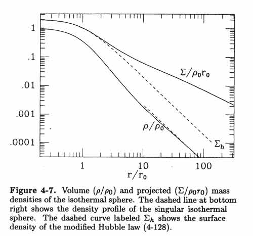
• We find a constant near-nuclear density : (r) ~ _o within a radius r_o = 3 / (4 G _o)^½
  This is a core and r_o is called the King (or core) radius
  I(r_o) = 0.5013 I(0), so r_o is appropriately defined
  r_o is also the scale length of the r^-2 envelope (see below): big cores are in big galaxies
  Circular velocity : V_c = - (d ln / d ln r)^½
  

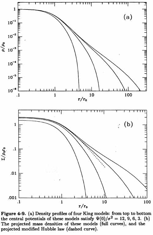
• When plotted as log ( / _o) vs log (r / r_o), there is only one isothermal profile

  • At small radii (e.g. r < few r_o)
    the density law resembles the Hubble density law : (r)     (1 + (r / r_o)²)^-3/2 = _H(r)
      I(R) fits ~OK to the centers of many Elliptical galaxies

  • At large radii (e.g. r 15 r_o)
    the system resembles the SIS : (r) (r / r_o)^-2   and   V_c = 2
    this is different from the Hubble density Law:
      projected light profile does not fit Ellipticals well in the outer parts (too flat)

• The scale length and central density together define the dispersion : ² _o r_o²
    for a given central density, hotter galaxies are larger
    for a given core radius, hotter galaxies are denser

• Quantitatively : ² = (4 / 9) G _o r_o²
  To simplify calculations, use G = 4.5 × 10^-3 in units of pc, km/s, and M
  Eg for = 100 km/s, r_o = 100 pc we have _o = 159 M pc^-3

• A good isothermal core match to the centers of Ellipticals can be used to estimate central M/L
    obtain r_o and I(0) from isothermal fits to I(R), and measure
  (express I(0) in units of L pc^-2 to allow simplified calculations with G = 4.5 × 10^-3)
  j(0) = 0.5 I(0) / r_o
  (0) = 9 ²/ (4 G r_o²)
  M/L = (0) / j(0)

  This method is called "core fitting" or "King's method"
  Typical values for ellipticals cores are 10-20 h M/ L suggesting minimal/no dark matter

• There is a problem with all isothermal models: they have infinite total mass
  It is easy to see why the system is at least infinite in extent :
  
  at any given radius, stars have isotropic dispersion
  at this radius at least some stars are therefore moving outward
  but further out the dispersion is still , and stars are moving outward
    the system must have infinite extent
  Ultimately, this arises because f(E_r) > 0 for negative E_r,   i.e. the model includes unbound stars.

  To rectify this problem, we attempt to modify things slightly by removing the unbound stars:  

• Suppress stars at large radius (ie as E_r 0,   we want f(E_r) 0)
  Modify the exponential DF:

  (8.35)

  where _o is a (dispersion like) parameter.

• Repeating the same analysis as before, we get for Poisson's eqn:

  (8.36)

  Solve this by integration, choosing boundary conditions at r = 0:
  

  (0) = q _o²     (q > 0, large q = deep central potential)
  d / dr = 0   (as before)

• Inner regions : like isothermal, with core (King) radius ~ r_o (defined as before)
  Outer regions : (r) decreases & approaches 0 at r_t
  Recall: velocity range at is 0     (2)
  So density = f d³v = 0 at r_t   = tidal or truncation radius = edge of sphere
  Larger (0) (larger q)     larger r_t & M_tot     M(r_t)
  Alternative parameter to (0) or q is concentration   c = log₁₀ (r_t / r_o)
  See: B&T fig 4.9, 4.10, 4.11   [images]

• Single sequence of King models by varying (equivalently): (0); q; c
  Empirically, we find:
  
  c = 0.75 - 1.75 ( q = 3 - 7)   fit GCs very well
  c > 2.2 ( q > 10)   fit some Ellipticals quite well
  c = 1.7 ( q = 8)   fits Hubble law well
  c = ( q = ) is the isothermal sphere

• King models are not isothermal : ² <v²> _o² within r_o but drops at larger radii.
  

The methods illustrated here can be applied to more complex systems:
Spherical systems with velocity anisotropy (B&T-2 4.3.2)
Axisymmetric systems (B&T-2 4.4)
Thin disks (B&T-2 4.5)

(9) Violent Relaxation

• The previous discussion focussed on static systems, since they are relatively tractable.
  Varying potentials are usually intractable and require a numerical approach.
  There are, however, a few situations which can be treated analytically
  Paradoxically, one of these is when the potential is maximally fluctuating
  This is the case of violent relaxation, which we now describe briefly

• For galaxies, 2-body encounters are negligible and evolution is determined by the CBE
  For a static potential, energy (E) of a star is conserved and the DF doesn't change
  Isolated galaxies in steady state do not, therefore, evolve dynamically
  (we're ignoring gas & 2-body processes here)

• For a galaxy to change, there needs to be a changing potential
  For each star, dE / dt   =   / t   at the star
  The DF evolves and the structure of the galaxy changes
  This occurs during (i) inhomogeneous collapse, and (ii) encounters (Topic 12)
  These are brief traumatic times :
    "galaxy changes are by revolution rather than by evolution"
  (nice quote from Binney's EAA article)

• In collapse of large cold system, changes rapidly
  Stars gain and lose energy, which broadens f(E)
  Energy is redistributed via collective interactions
  This acts like a relaxation process [image & movie].

• N-Body example: van Albada 1982 (B&T 4.7.3)   ([images] : B&T figs 4.19-22)
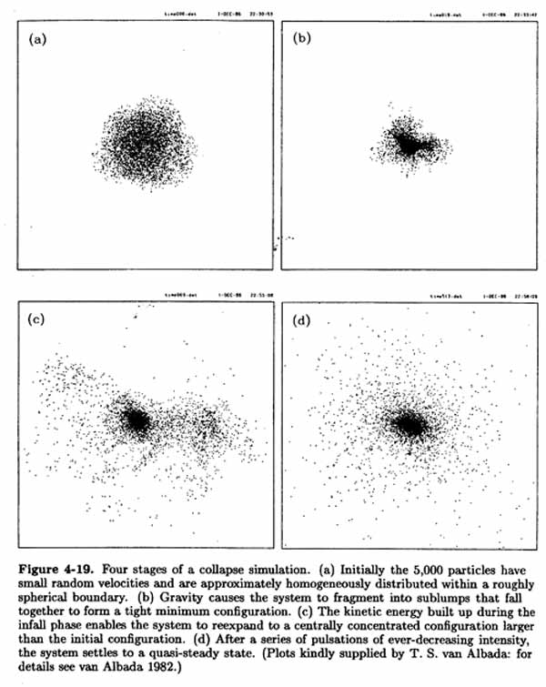  Start with ~ homogeneous sphere with low   (Similar to Klypin simulation above).
  1st infall: clumps grow; infall speeds up; dense inhomogeneous center; much scattering
  Rebound: stars fly back out; some lost; many stay near center
  Oscillations die down; system settles into ~ R^¼ law; with decreases outwards
  Anisotropy, , is 0 at nucleus,     1 at edge
  (Most scattering occurs at small r on 1st infall     most stars have low AM
  N(E) dE spreads out, most stars have E ~ 0, few are deeply bound
  

• Note: the total energy remains constant : this is a non-dissipational process
  energy is not radiated away, as with dissipational (gaseous) collapse
  If the total energy is initially zero (eg diffuse system at rest), then following collapse :
  some stars will be strongly bound, but some must also have been ejected.

• Note: scattering is independent of the star's mass
  fundamentally different from 2-body relaxation
  no segregation by mass (eg heavy stars don't sink to center)
  

• Phase mixing helps smooth out lumps fairly quickly
  distribution is ~smooth after ~few collapse times
    violent relaxation timescale is ~few × dynamical (collapse) timescale

• If relaxation is complete, then fully random scattering occurs
    results in isotropic velocity field and Boltzmann-like f(E)
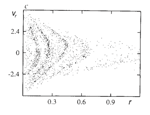
  Usually, however, the density distribution becomes smooth before scattering is complete.
  Relaxation ceases and is incomplete
    residual anisotropies & phase-space substructures [images & movie]

  

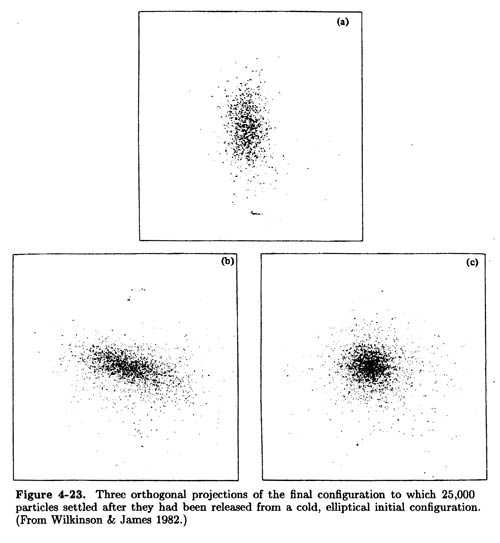
• If the initial distribution is hotter     less concentrated
  If the initial distribution is rotating slowly     less concentrated & rotating oblate figure
  If the initial distribution is rotating faster     even less concentrated & prolate/bar figure
  If the initial distribution is ellipsoidal     rotating ellipsoid, anisotropic everywhere [image]
  

(10) Introducing Star-Star Encounters

• As usual : mean free path   =   1 / nA     and time between encounters   =   1 / nAV
  for encounter crossection A ~ b²   (b = impact parameter); star density n; and mean velocity V
  We consider three regimes :

  (i) Direct collision (or tidal capture)

• For b ~ few × R_star strong tides dissipate orbital energy, leading to tidal capture
  depending on circumstances, the stars may ultimately coalesce
    this is exceedingly rare in present day galaxies
  

  (ii) Strong Deflection

• Defined as V V     occurring when   b r_s   (s for strong) is sufficiently small
  from virial theorem :   G m² / r_s ~   m V²     so     r_s   ~   G m / V²   (here m is star mass)
    this is   ~ 1 AU for the sun, using V ~ 20 - 30 km/s 
  (cf V for earth's orbit _* in solar neighborhood)

• The interval, t_s, between collisions = 1 / n r_s² V   =   V³ / (G²m² n)   ~ 10¹⁵ years for sun
     this is very rare for most stellar systems
  may be relevant in dense GC nuclei, galactic nuclei and galaxy clusters 

  (iii) Weak Deflection

• Defined as V << V     so b   >> r_s
  estimate deflection velocity towards target star : [image]
  time in vicinity of target star :   t 2b / V
  acceleration     Gm / b²     so V 2Gm / bV
  Angle of deflection V / V   2Gm / bV²   2 arcsec in solar neighborhood
  

• After many encounters :   V_tot = V
  since the direction of pull is random, V_tot executes a random walk
  the amplitude (squared) of this resultant velocity after time t is given by :

  (8.37a)        (8.37b)

  where = b_max / b_min

• The system has relaxed when the velocity changes by ~100%, ie when V_tot V
  Integrating over a Maxwellian changes the numerical constant slightly (B&T §8.4)
  Changing V to , and writing m n as , the stellar density, we get (B&T eq 8-71)

  (8.38a)         (8.38b)

  where ₁₀ has units 10 km/s, m has units of M, and ₃ has units 10³ M / pc³
  

• There is a surprisingly simple alternative expression for the relaxation time
  It is less precise but is adequate in many circumstances
  We start, as before, with equation 8.37b :
  For a system of size R containing N stars :   n = 3N / (4R³)
  From the virial theorem :   V² = GM / R   =   GNm / R
  The system relaxes when V_tot V
  Take b_max R;   b_min r_s = Gm / V²,   so b_max / b_min = = N
  Choose units of time :   t = t_cross R / V
  

  Substituing, we get

  (8.38c)

• Surprisingly, this only depends on N, the total number of stars in the system

• Notice that t_relax > t_cross   for   N 30
    to good approximation, stars usually orbit in the overall potential

• Equal logarithmic intervals in b contribute equally to long term deflection.
  E.g. the ranges : R to ½R ;   ½R to ¼R ; ....... 2b_min to b_min   all contribute equally

• However, since the deflection drops rapidly with b as V / V 1 / b
    for systems with R >> b_min most scattering is due to weak encounters (V << V)
  Example :
  Galaxy with R ~ 10 kpc ; b_min ~ 1 AU (1 M stars); so ln = 20
  Half deflection from encounters outside b₁ where ln R/b₁ = 10
  3/4 deflection from encounters outside b₂ where ln R/b₂ = 15
  b₁ = 0.5 pc for which V / V = b_min / b₁ 10^-5  
  b₂ = 0.003 pc for which V / V = b_min / b₂ 0.15%  

• Need care with N-Body simulations when N << N_stars
  is more grainy than reality, and t_relax(simulation) << t_relax(reality)
  Avoid by softening star potentials to increase b_min
  Care: lose structure on scales R < b_min

(b) Timescales for Real Stellar Systems

• Here are rough timescales (in years) for a number of stellar systems :
  

  System	N	R (pc)	V (km/s)	tcross	trelax	tage	age/relax
  Open Cluster	102	2	0.5	106	107	108	10
  Globular Cluster	105	4	10	5 ×105	4 ×108	1010	20
  Dwarf Galaxy	109	103	50	2 ×107	1014	1010	10-4
  Elliptical	1011	104.5	250	108	4 ×1016	1010	10-7
  Spiral Disk	1011	104.5	20	1.5 ×109	6 ×1017	1010	10-8
  MW Nucleus	106	1	150	104	108	1010	100
  Luminous Nucleus	108	10	500	2 ×104	1010	1010	1
  (Galaxy Cluster)	102	5 ×105	500	109	(3 ×109)	1010	(3)

• The presence of dark matter complicates the situation in clusters (see [Topic 13.4c])
  In practice, 2-body relaxation is not as fast as our simple analysis suggests.

• 2-Body relaxation may be relevant for star clusters and galaxy nuclei.

• For most galaxies, 2-body relaxation is utterly negligible.
  Because this course deals specifically with galaxies (and not star clusters)
  We will only briefly consider the ramifications of relaxation.

• Don't forget, relaxation times can vary greatly within a given system
  For example, a GC core can be relaxing while the halo is not.

• You may be wondering when Max Planck (& Adriaan Fokker) worked on stellar dynamics....
  They didn't : much of this work has its roots in plasma physics
  Unlike neutral gases, charges in plasmas have long range Coulomb interactions
  The early work on plasmas has been appropriated and applied to stellar systems
  

• For a smooth potential, the DF obeys the CBE : df / dt = 0
  With encounters, stars scatter into and out of the phase space trajectory:  df / dt = (f)
  (f) is a collision term and itself depends on f
  

• If the full collision term is included we have the master equation.
  If most scatterings are distant, an approximation for the collision term yields the Fokker-Planck equation.
  This is a PDE, for which several approaches to solutions have been made (see B&T-2 7.4).

(i) Relaxation

• 2-body relaxation introduces the equivalent of thermal conduction in a gas
  For self-gravitating systems, this can be a rather interesting process
  Recall from [§8.5e] that such systems have negative specific heat
    if you remove energy (heat), stars fall deeper in the gravitational well
    they therefore speed up, and that part of the system gets hotter

• In its simplest form, this relaxation renders clusters more centrally concentrated
    stellar encounters in the core pass energy to envelope stars
    the core contracts and heats, the envelope expands and cools
  After some time the envelope develops a density profile (r) r^-3.5
  Radial anisotropy increases with time and radius
  (stars kicked out from encounters in the core, so carry little AM)
  A successful DF is due to Michie, and is f(E,L) exp(-L²/L_o²) × [exp(E / ²) - 1]

• After about 15 t_relax, the process takes off in a runaway gravothermal catastrophe
  (An intuitive explanation is tricky -- see B&T-2 7.3.2)
  This "event" is called core collapse and leaves a density law (r) r^-2.23 (infinite at r=0 !)
  Since GC are about 20 × t_relax old, at least some have probably undergone core collapse
  In practice, core collapse is not as dramatic as its name suggests :
  Either
  • The core "runs out of stars" before densities become exotic
  • A hard binary forms which
      (a) ejects stars from the system, accelerating evaporation
      (b) scatters core stars, heating the core and halting core collapse
              (binary acts like nuclear burning in a star)

  (ii) Equipartition

• Violent relaxation during formation leaves all stars the same velocity distribution
  Consequently heavier stars have more kinetic energy.
  This is unlike a gas, where molecules have the same kinetic energy (heavier ones move slower).

• 2-body encounters mimic molecular interactions: energy passed from high mass to low mass stars
  In the limit of complete interaction, energy is shared equally (hence equipartition)

• More massive stars begin to sink deeper     mass segregation.
  Probably occurred in GCs, though difficult to check since (visible) giants all have similar mass.
  May have played role in galaxy clusters, but complicated by other effects (dynamical friction, mergers).

  (iii) Escape (Ejection and Evaporation)

• Encounters can result in stars with V > V_esc
  This can occur in two ways :
  A single encounter gives the star sufficient energy to escape (ejection)
  A star slowly wanders into unbound phase space due to many distant encounters
  From the analysis above (10.a.iii), the second is much more important

• Using the fact that V_esc² = -2(r),   it is easy to show (B&T p 490) that <V_esc²> = 4 <V²>
  So the rms escape velocity is just twice the rms velocity
  For a Maxwellian, the fraction with V > 2V_rms = 7 ×10^-3
  So this fraction is lost every t_relax     t_evap 140 t_relax
  

• The process speeds up in a galaxy tidal field, since V_esc is reduced (see [Topic 12.3.b])

• Evaporation + equipartition   less massive stars evaporate first (higher velocities).
  Explains unusually low M/L (~2) for GCs compared to other pop II objects (M/L ~ 10).

• The observed distribution of t_relax for the ~150 MW GCs shows essentially none < 10⁸ years
  Selection effect: since t_evap ~ 100 t_relax these GCs have probably already evaporated
  Suggests young MW may have had many more GCs

(11) Further Topics

• Dynamical Friction [ Topic 12 § 3a ]
• Tidal Evaporation [ Topic 12 § 3b]
• Slow (adiabatic) & Fast (impulsive) Encounters [ Topic 12 § 3c]
• Mergers [ Topic 12 § 3d]
• The effects of central black holes on galaxy nuclei [ Topic 14 § 5]