Dynamic Range of a Receiver
beginning
distortion
minimum
sensitivity
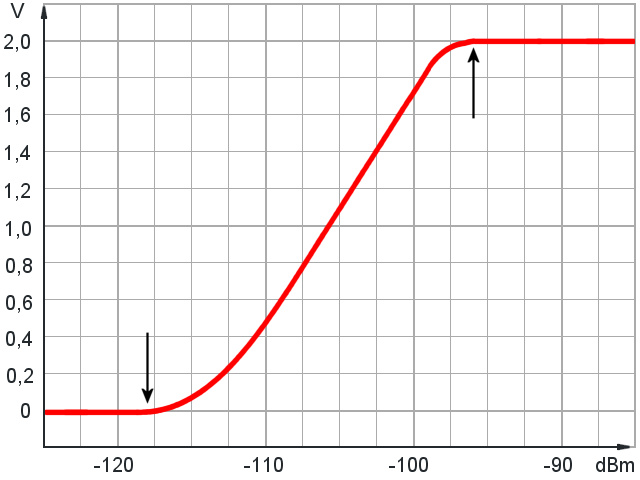
Figure 1: A so-called Receiver-Calibration Curve: The output signal (Y-axis) is a function of the receiver input power (X-axis). The difference between the point of beginning distortion and the point of the minimum sensitivity isf the dynamic range of the receiver in Decibel (here: 118 - 83 = 35 dB).
beginning
distortion
minimum
sensitivity
Figure 1: A so-called Receiver-Calibration Curve: The output signal (Y-axis) is a function of the receiver input power (X-axis). The difference between the point of beginning distortion and the point of the minimum sensitivity isf the dynamic range of the receiver in Decibel (here: 118 - 83 = 35 dB).
Dynamic Range of a Receiver
The power ratio between the echo signals from close range and the echo signals of objects from a very large distance can be up to 80 dB. Signals with such large power differences can be processed very difficult. This applies particularly if the echo signals are to be converted to digital data format later in the radar signal processing.
The term “dynamic” describes the ratio between maximum and minimum possible received power of a receiver without the receiver being driven in the overload. For radar receiver following values approach is required:
| D = | Prmax | = value of maximum signal power, in which the receiver is not overloaded. = value of minimum signal power, in which the receiver still issues an output signal. | |
| Prmin |
Most radar parameters from the radar equation can be viewed to be constant within a pulse period. There are only the radar cross-section σ and the respective distance of the target to be localized but highly variable. Therefore can be considered the minimum as possible received power in proportion to the smallest reflection surface in the maximum possible distance, and vice versa, the maximum expected received power from a target with a very large effective reflection area in the minimum possible measurement distance.
| Pr = | Pt λ2 G2 σ | = k · | σ | (2) |
| (4π)3 · R4 | R4 |
The relatively constant values in the radar equation are combined to form a constant factor k, and this one is then truncated mathematically:
| D = | Prmax | = | k · σmax / R4min | = | σmax · R4max | (3) |
| Prmim | k · σmin / R4max | σmin · R4min |
If in this formula used real data of a given radar set, we obtain the required dynamic range of the receiver. For example, the ATC-radar ASR-E by the duration of the transmit pulse of 45 microseconds (the internal modulated pulse for long-range) a minimum range of 6.75 km. The maximum range with the same transmit pulse, thus specified by 60 nautical miles, i.e. 110 km. Rhe receiver should be able to process radar cross-sections of a minimum of 0.1 m² (ultralight aircraft) to a maximum of 100 m² (big cargo plane):
| D = | 100 m² · (110 km)4 | = 7 · 107 ≈ 78.5 dB |
| 0.1 m² · (6.75 km)4 |
Thus the receiver needs a dynamic range of 78.5 dB. It must be able to process in addition to the smallest possible echo signal also these echo signals, which are 70 million times larger.
This is not possible without few circuit tricks that allow a so-called dynamic compression. It should be noted that this compression must be done true to scale: The amplitude differences must be mathematically traced back later!