Intrapulse Modulation and Pulse Compression
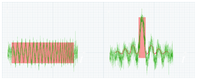
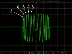
Figure 1: Input and output signals of a pulse compression stage, the received signal in noise is hardly noticeable, so the pulse compression results in a clear echo signal.
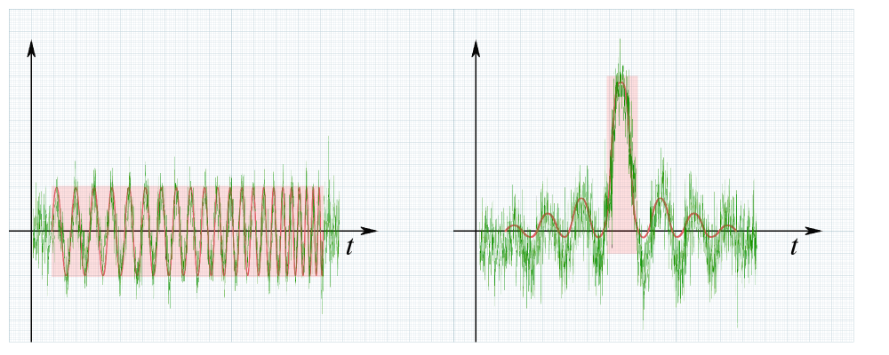
Figure 1: Input and output signals of a pulse compression stage, the received signal in noise is hardly noticeable, so the pulse compression results in a clear echo signal.
Figure 1: Input and output signals of a pulse compression stage, the received signal in noise is hardly noticeable, so the pulse compression results in a clear echo signal.
Intrapulse Modulation and Pulse Compression
Pulse compression is a generic term that is used to describe a waveshaping process that is produced as a propagating waveform is modified by the electrical network properties of the transmission line. The pulse is internally modulated in phase or in frequency, which provides a method to further resolve targets which may have overlapping returns (so-called Intrapulse Modulation). Pulse compression originated with the desire to amplify the transmitted impulse (peak) power by temporal compression. It is a method which combines the high energy of a long pulse width with the high-resolution of a short pulse width. The pulse structure is shown in figure 1.
Pulse radar sets of the older type require a high pulse power to achieve the desired range. At the same time the transmission pulse should be as short as possible, because this parameter affects the range resolution. These radars must are able to generate and radiate the total transmit power in just a few micro- or even nanoseconds. For this task have been developed powerful modulator and transmitter vacuum tubes.
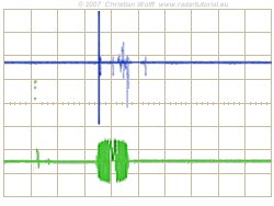
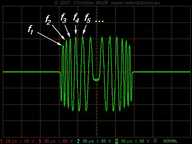
Figure 2: short pulse (blue) and a long pulse with intrapulsemodulation (green)
In semiconductor technology made high-power transmitters (transmitter in solid-state technology) are not able to produce such high-power pulses due to their limited dielectric strength and its limited working temperature. To radiate the same transmission energy, the transmitting pulse of this radar must therefore be much longer. In order to improve range resolution of radar pulse having a relatively large transmitting pulse duration, the pulse is modulated internally. Since each part of the pulse has unique frequency, these returns can be completely separated and integrated into a shorter single output pulse. The echo signal is therefore compressed in its pulse duration in special filters. The procedure for this is called pulse compression. Now it is possible to perform a localization within the transmitted and now received pulse. In pulse compression, the energetic advantages of very long pulses with the benefits of very short pulses are combined. Through the necessary modulation self-oscillating channels cannot perform this procedure.
The noise in the receiver is always broadband with a random distribution. The frequency synchronous amount of the received noise is rather low compared to the echo signal. The amount of noise is greatly reduced by the pulse compression filter therefore. Thus, by the pulse compression can be achieved even then an output signal when the input signal is smaller than the noise floor and would be lost for a simple diode demodulation.
This modulation or coding can be either
- FM (frequency modulation)
- linear (chirp radar) or
- non-linear,
- time-frequency-coded waveform (e.g. Costas code) or
- PM (phase modulation).
Now the receiver is able to separate targets with overlapping of noise. The received echo is processed in the receiver by the compression filter. The compression filter readjusts the relative phases of the frequency components so that a narrow or compressed pulse is again produced. The radar therefore obtains a better maximum range than it is expected because of the conventional radar equation.
The ability of the receiver to improve the range resolution over that of the conventional system is called the pulse compression ratio (PCR). For example a pulse compression ratio of 50:1 means that the system range resolution is reduced by 1/50 of the conventional system. The pulse compression ratio can be expressed as the ratio of the range resolution of an unmodulated pulse of length τ to that of the modulated pulse of the same length and bandwidth B.
| PCR = | (c0 · τ /2) | = B · τ | (1) |
| (c0 / 2B) |
This term is described as time-bandwidth product of the modulated pulse and is equal to the Pulse Compression Gain, PCG, as the gain in SNR relative to an unmodulated pulse. Alternatively, the factor of improvement is given the symbol PCR, which can be used as a number in the range resolution equation, which now achieves:
| Rres = c0 · (τ / 2) = PCR · c0 /2 B | (2) |
The compression ratio is equal to the number of sub pulses in the waveform, i.e., the number of elements in the code. The range resolution is therefore proportional to the time duration of one element of the code. The radar maximum range is increased by the fourth root of PCR.
The minimum range is not improved by the process. The full pulse width still applies to the transmission, which requires the duplexer to remained aligned to the transmitter throughout the pulse. Therefore Rmin is unaffected.
| Advantages | Disadvantages |
| lower pulse-power therefore suitable for Solid-State-amplifier | high wiring effort |
| higher maximum range | bad minimum range |
| good range resolution | time-sidelobes |
| better jamming immunity | |
| difficulter reconnaissance |
Table 1: Advantages and disadvantages of the pulse compression
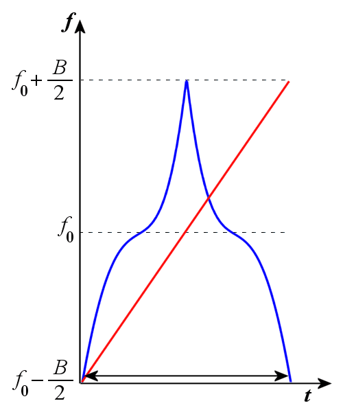
Pulse compression with linear FM waveform
At this pulse compression method the transmitting pulse has a linear FM waveform. This has the advantage that the wiring still can relatively be kept simple. However, the linear frequency modulation has the disadvantage that jamming signals can be produced relatively easily by so-called “Sweeper”.
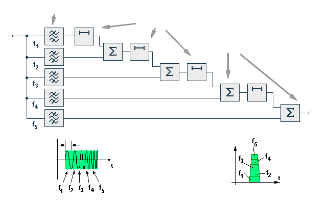
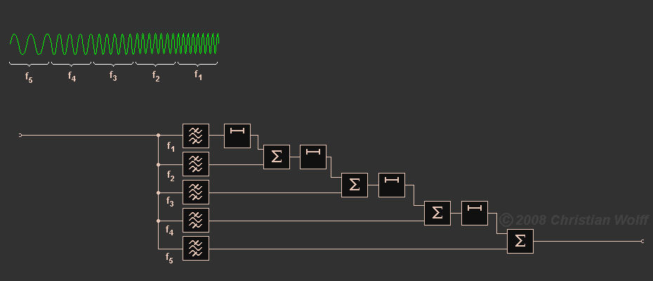
The block diagram on the picture illustrates, in more detail, the principles of a pulse compression filter.

a frequency component
Figure 3: Block diagram (an animation as explanation of the mode of operation)
a frequency component
Figure 3: Block diagram
a frequency component
Figure 3: Block diagram (an animation as explanation of the mode of operation)
The compression filter are simply dispersive delay lines with a delay, which is a linear function of the frequency. The compression filter allows the end of the pulse to „catch up” to the beginning, and produces a narrower output pulse with a higher amplitude.
As an example of an application of the pulse compression with linear FM waveform can be mentioned the air defence radar AN/FPS-117 .
Filters for linear FM pulse compression radars are now based on two main types.
- Digital processing (following of the A/D- conversion).
- Surface acoustic wave devices.
(angularly)
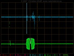
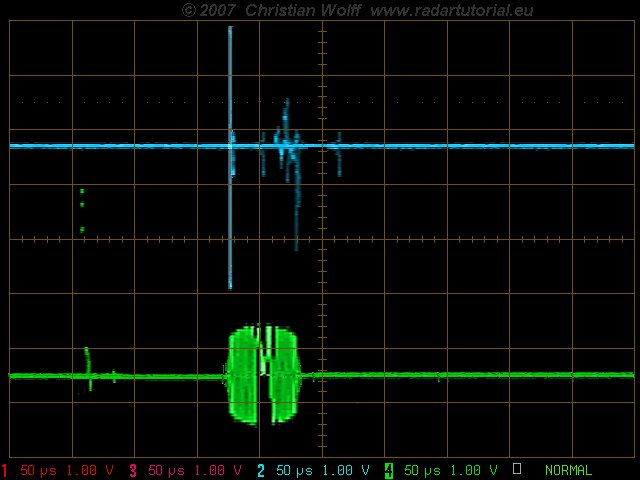
Figure 4: View of the time side lobes at an oscilloscope (upper figure) and at B-scope
(angularly)
Figure 4: View of the time side lobes at an oscilloscope (upper figure) and at B-scope
Time-Side-Lobes
The output of the compression filter consists of the compressed pulse accompanied by responses at other times (i.e., at other ranges), called time or range sidelobes. The figure shows a view of the compressed pulse of a chirp radar at an oscilloscope and at a ppi-scope sector.
Amplitude weighting of the output signals may be used to reduce the time sidelobes to an acceptable level. Weighting on reception only results a filter „mismatch” and some loss of signal to noise ratio.
The sidelobe levels are an important parameter when specifying a pulse compression radar. The application of weighting functions can reduce time sidelobes to the order of 30 db's.
Pulse compression with non-linear FM waveform
The non-linear FM waveform has several distinct advantages. The non-linear FM waveform requires no amplitude weighting for time-sidelobe suppression since the FM modulation of the waveform is designed to provide the desired amplitude spectrum, i.e., low sidelobe levels of the compressed pulse can be achieved without using amplitude weighting.
Matched-filter reception and low sidelobes become compatible in this design. Thus the loss in signal-to-noise ratio associated with weighting by the usual mismatching techniques is eliminated.
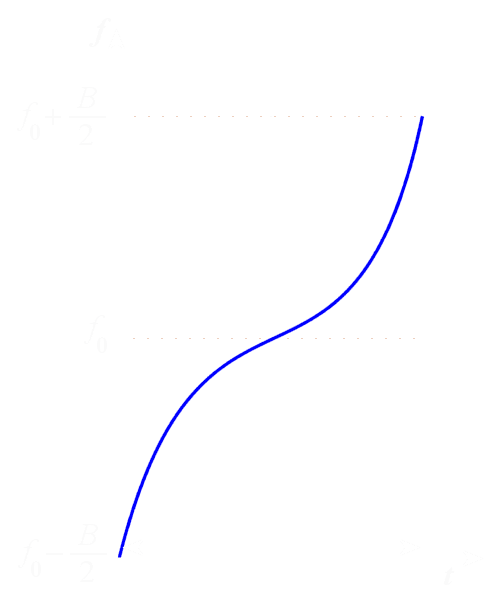
A symmetrical waveform has a frequency that increases (or decreases) with time during the first half of the pulse and decreases (or increases) during the last half of the pulse. A non symmetrical waveform is obtained by using one half of a symmetrical waveform.
The disadvantages of the non-linear FM waveform are
- Greater system complexity
- The necessity for a separate FM modulation design for each type of pulse to achieve the required sidelobe level.
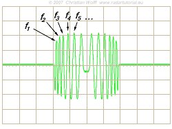
Figure 6: A non-symmetrical waveform (Output of the Waveform-Generator)
symetrically
Figure 5: symetrically waveform
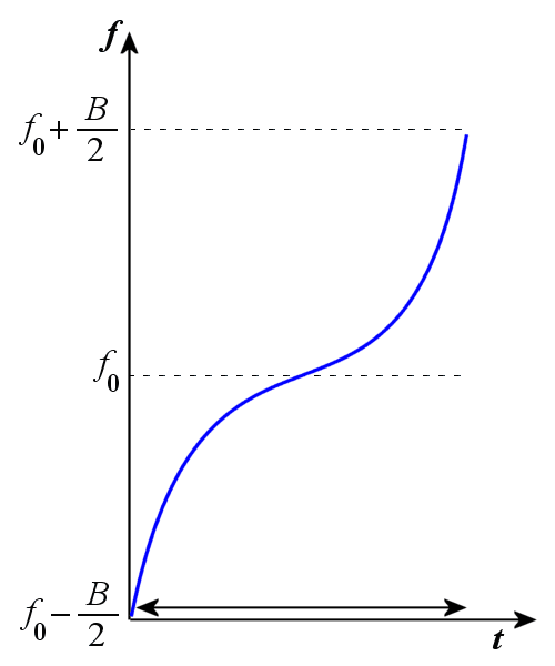
Figure 7: non-symetrically waveform
Phase-Coded Pulse Compression
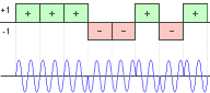
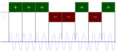
Figure 8: diagram of a phase-coded pulse compression
Phase-coded waveforms differ from FM waveforms in that the long pulse is sub-divided into a number of shorter sub pulses. Generally, each sub pulse corresponds with a range bin. The sub pulses are of equal time duration; each is transmitted with a particular phase. The phase of each sub-pulse is selected in accordance with a phase code. The most widely used type of phase coding is binary coding.
The binary code consists of a sequence of either +1 and -1. The phase of the transmitted signal alternates between 0 and 180° in accordance with the sequence of elements, in the phase code, as shown on the figure. Since the transmitted frequency is usually not a multiple of the reciprocal of the sub pulsewidth, the coded signal is generally discontinuous at the phase-reversal points.
| Length of code n | Code elements | Peak-sidelobe ratio, dB |
| 2 | +- | -6.0 |
| 3 | ++- | -9.5 |
| 4 | ++-+ , +++- | -12.0 |
| 5 | +++-+ | -14.0 |
| 7 | +++--+- | -16.9 |
| 11 | +++---+--+- | -20.8 |
| 13 | +++++--++-+-+ | -22.3 |
Table: Barker Codes
The selection of the so-called random 0, π phases is in fact critical. A special class of binary codes is the optimum, or Barker, codes. They are optimum in the sense that they provide low sidelobes, which are all of equal magnitude. Only a small number of these optimum codes exist. They are shown on the beside table. A computer based study searched for Barker codes up to 6000, and obtained only 13 as the maximum value.
It will be noted that there are none greater than 13 which implies a maximum compression ratio of 13, which is rather low. The sidelobe level is -22.3 db.