Antenna Pattern
level
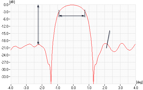
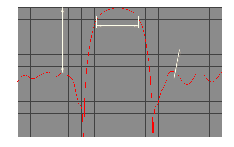
Figure 1: Example antenna pattern of an Large Vertical Aperture (LVA) in a Cartesian coordinate system
level
Figure 1: Example antenna radiation pattern of an LVA in a Cartesian coordinate system
The term antenna pattern (or radiation pattern) most commonly refers to the directional (angular) dependence of radiation from the antenna. It is the geometric pattern of the relative strengths of the field emitted by the antenna. Very often, only the relative amplitude is plotted, normalized either to the amplitude on the antenna boresight. As a consequence of the reciprocity theorem, the receiving pattern (sensitivity as a function of direction) is identical to the relative power density of the wave transmitted by the same antenna (power density as a function of direction). The pattern of an antenna may be determined experimentally at an antenna range, or alternatively, deduced by computation. The plots of the antenna pattern can be used to benchmark a given radar antenna. They also tell you how much degradation you can expect if the antenna is not aimed properly.
For the ideal isotropic antenna, the transmitted power density is equally in all directions, the plot of the antenna pattern would be formed as a sphere. Directional antennas like radar antennas provide a greater concentration of radiation in one desired direction. The radar achieves a longer range in this direction with a focused, narrow radio wave beamwidth. This narrow beamwidth allows more precise targeting of the echo-signal. The radiation pattern is a graphical depiction of the measured relative field strength transmitted from or received by the antenna. In the radiation pattern, the distance of the surface from the origin is proportional to the magnitude of the E field at some fixed distance from the antenna in the corresponding direction.
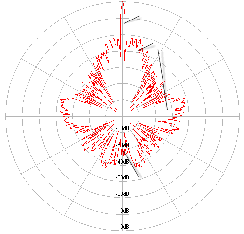
Figure 2: Horizontal cross-section of the radiation pattern in a polar coordinate system
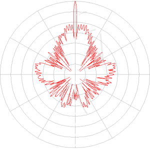
Figure 2: Horizontal cross-section of the radiation pattern in a polar coordinate system
Horizontal Radiation Pattern
The radiation pattern of an antenna is typically represented by a three-dimensional graph. Radiation plots are most often shown in either the plane of the axis of the antenna or the plane perpendicular to the axis and are referred to as the azimuth and the elevation respectively. The graphs can be drawn using Cartesian (rectangular) coordinates or a polar plot. Each format has its own advantages and disadvantages. In a Cartesian coordinate system, the detail is good but the pattern shape is not always apparent. This type of plot was preferred when the exact level of the side lobes is important. The computer-aided plots provide a table with the exact levels too. The polar coordinate system is more compatible with maps and provides a quick reference to the response of the antenna in any direction. The antenna supplier either measures the radiation pattern by rotating the antenna on its axis or calculates the signal strength around the points of the compass with respect to the main beam peak.
While a graphic in Polar-coordinates may be useful for visual inspections, it may not be useful for an engineering analysis task. So the measured or computed data may also be exported in numerical values in a table format.
Vertical Radiation Pattern
The shape of the vertical pattern is a vertical cross cut of the three-dimensional graph. In the shown polar diagram (a quarter part of the circle) with the antenna site as the origin, the x-axis is the radar range, and the y-axis the aims height. One of the antenna measurement techniques is the Sun-Strobe-Recording using RASS-S, a measurement tool of Intersoft Electronics. The RASS-S (Radar Analysis Support System for Sites) is a radar manufacturer-independent system for evaluating the different elements of radar by connecting to signals which are already available and this under operational conditions.
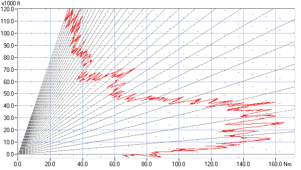
Figure 3: Vertical antenna pattern with cosecant-squared characteristic
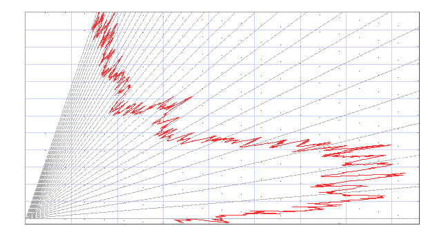
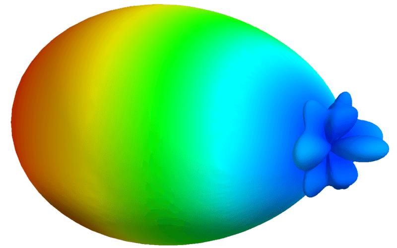
Figure 4: Three-dimensional antenna pattern of a feedhorn
Figure 4: Three-dimensional antenna pattern of a feedhorn
In the shown Figure 3, the measurement units are nautical miles as range, and feet as height. Both measurement units are still used in Air- Traffic- Management by historical reasons. These units are of secondarily meaning only because the plotted quantity of radiation pattern is defined as a relative level. This means the boresight axis has got the value of the (theoretical) maximum range calculated with the help of the Radar Equation. The shape of the plot provides the required information only! To get absolute values you need a second plot, measured under the same conditions. These two plots you can compare and then you achieve over increasing or decreasing the antennas performance.
The radiant lines are marks of elevation angles, here in half-degree-steps. The unequal scales of the x-axis and the y-axis (many feet versus a lot of nautical miles) cause the non-linear spacing between the elevation angle marks. The height is shown as a linear grid pattern. A second (dotted) grid is orientated on the curvature of the earth.